Modelling Data using Functions
Learning Outcomes
After learning through these examples, you will be able to:
- Apply the principle of least squares.
- Use the procedure for fitting any curve or functional relationship.
- Calculate the residuals.
- Fit a straight line to the given data.
- Fit a second-degree parabola to the given data.
- Fit a power curve \(Y = aX^b\) to the given data.
- Fit exponential curves of the forms \(Y = ab^X\) and Y = \(ae^X.\)
- Visualize the data using a scatter plot and the best-fitted line/curve in the same figure.
- Use the
Rbuilt-in functionlmto check your numerical computations. - Learn
Rcode to import the data, plot the figures, and use theRbuilt-in functions.
Learning Modes
The first eight worked examples demonstrate the principle of least squares through a procedural learning approach. These examples include the best-fitting linear, second-degree, power curve, and exponential curve forms.
In a multiple-choice format, you will engage with various interactive elements, such as buttons to click and select, as well as options to rearrange boxes in a logical flow. Four questions are designed to test your understanding and application of modeling data using these functions. A timer will also track how long it takes you to solve these problems.
At the end of this section, suggested solutions for the four problems will be provided for you to check your answers.
1 Example 1
Find a straight line that best fits the following data:
\[ \begin{array}{c|cccccccccccc} x & 1 & 6 & 11 & 16 & 20 & 26 \\ \hline y & 13 & 16 & 17 & 23 & 24 & 31 \end{array} \] Solution
Let the straight line be given by the equation \(Y = a + bX\). To determine the values of \(a\) and \(b\) for this line, we use the normal equations:
\[ \begin{array}{cccccc} \displaystyle \sum_{i=1}^{n} y_i &=& na & + &\displaystyle b \sum_{i=1}^{n} x_i \\ \displaystyle \sum_{i=1}^{n} y_i x_i &= & a\displaystyle\sum_{i=1}^{n}x_i & + & \displaystyle b\sum_{i=1}^{n}x_i^{2} \end{array} \]
can be written as
\[ \begin{array}{cccccc} \displaystyle \sum y & = &na &+& \displaystyle b \sum x \\ \displaystyle \sum yx & = & \displaystyle a \sum x &+& \displaystyle b \sum x^{2} \end{array} \]
We need to calculate \(\displaystyle \sum y\), \(\displaystyle \sum x\), \(\displaystyle \sum xy\), and \(\displaystyle \sum x^2\), which can be obtained from the following table:
\[ \begin{array}{ccccccccccccc} i & x & y & x^2 & xy \\ \hline 1 & 1 & 13 & 1 & 13 \\ 2 & 6 & 16 & 36 & 96 \\ 3 & 11 & 17 & 121 & 187 \\ 4 & 16 & 23 & 256 & 368 \\ 5 & 20 & 24 & 400 & 480 \\ 6 & 26 & 31 & 676 & 806 \\ \hline n = 6 & \displaystyle \sum x = 80 & \displaystyle \sum y = 124 & \displaystyle \sum x^2 = 1490 & \displaystyle \sum xy = 1950 \\ \hline \end{array} \]
For example, \[\begin{align*} \displaystyle \sum x & = \sum_{i=1}^6 x_i \\ & = x_1 + x_2 + x_3 + x_4 + x_5 + x_6 \\ & = 1 + 6 + 11 + 16 + 20 + 26 \\ & = 80, \end{align*}\] \[\begin{align*} \displaystyle \sum y & = \sum_{i=1}^6 y_i \\ & = y_1 + y_2 + y_3 + y_4 + y_5 + y_6 \\ & = 13 + 16 + 17 + 23 + 24 + 31 \\ & = 124, \end{align*}\] \[\begin{align*} \displaystyle \sum y & = \sum_{i=1}^6 x_i^2 \\ & = x_1^2 + x_2^2 + x_3^2 + x_4^2 + x_5^2 + x_6^2 \\ & = 1^2 + 6^2 + 11^2 + 16^2 + 20^2 + 26^2 \\ & = 1 + 36 + 121 + 256 + 400 + 676 \\ & = 1490, \end{align*}\] and \[\begin{align*} \displaystyle \sum xy & = \sum_{i=1}^6 x_i y_i \\ & = x_1 y_1 + x_2 y_2 + x_3 y_3 + x_4 y_4 + x_5 y_5 + x_6 y_6 \\ & = 13 + 96 + 187 + 368 + 480 + 806 \\ & = 1950 \end{align*}\]
By substituting the values of \(\displaystyle \sum y\), \(\displaystyle \sum x\), \(\displaystyle \sum xy\), and \(\displaystyle \sum x^2\) into the normal equations, we obtain:
\[ \begin{array}{cccccc} \displaystyle 124 & =& 6 a &+& 80 b && (1)\\ \displaystyle 1950 & = &80 a &+& 1490 b && (2) \end{array} \] Now we solve equations (1) and (2).
Multiplying equation (1) by 80 and equation (2) by 6, i.e.
\[ \begin{array}{cccccc} \displaystyle 124 & =& 6 a &+& 80 b && \times \quad 80 \\ \displaystyle 1950 & =& 80 a &+& 1490 b && \times \quad 6 \end{array} \] we have \[ \begin{array}{cccccc} \displaystyle 9920 & = & 480 a &+& 6400 b && (3) \\ \displaystyle 11700 & = & 480 a &+&8940 b && (4) \end{array} \]
Subtracting (3) from (4), we obtain
\[ \begin{array}{ccllll} \displaystyle & 1780 & = & 2540 b & & \\ \displaystyle \Rightarrow & b & = & 1780/2540 & =& 0.7008 \end{array} \]
By substituting the value of \(b\) in equation (2), we have
\[ \begin{array}{ccclll} & 24 & = & 6a+80\times 0.7008 \\ & 124 & = & 6a+56.064 \\ & 67.936 & = & 6a \\ \Rightarrow & a & = & 11.3227 \end{array} \]
with these values for \(a\) and \(b\), the equation for the line of best fit is: \(Y=11.3227+0.7008 X\).
# Create a data frame to store the data
X <- c(1,  6, 11, 16, 20, 26)
Y <- c(13, 16,  17, 23, 24, 31)
data <- data.frame(X, Y)
data| X | Y |
|---|---|
| 1 | 13 |
| 6 | 16 |
| 11 | 17 |
| 16 | 23 |
| 20 | 24 |
| 26 | 31 |
# Create a scatterplot of Y versus X
plot(
  data$X,
  data$Y,
  main = "Y vs. X",
  xlab = "X",
  ylab = "Y"
  )

# Fit a linear regression model to the data
linear_model <- lm(Y ~ X, data = data)

# Summarize the linear regression model
summary(linear_model)
##
## Call:
## lm(formula = Y ~ X, data = data)
##
## Residuals:
## 1 2 3 4 5 6
## 0.9764 0.4724 -2.0315 0.4646 -1.3386 1.4567
##
## Coefficients:
## Estimate Std. Error t value Pr(>|t|)
## (Intercept) 11.32283 1.17618 9.627 0.000651 ***
## X 0.70079 0.07464 9.389 0.000717 ***
## ---
## Signif. codes: 0 '***' 0.001 '**' 0.01 '*' 0.05 '.' 0.1 ' ' 1
##
## Residual standard error: 1.536 on 4 degrees of freedom
## Multiple R-squared: 0.9566, Adjusted R-squared: 0.9457
## F-statistic: 88.16 on 1 and 4 DF, p-value: 0.0007169# Calculate the predicted Y for a range of X
predicted_values <- predict(
linear_model,
newdata = data.frame(X = seq(min(X),
max(X),
length.out = 5)
)
)
# Plot the data points and the predicted Y values
plot(
data$X,
data$Y,
main = "Y vs. X",
xlab = "X",
ylab = "Y"
)
lines(seq(min(X),
max(X),
length.out = 5),
predicted_values, col = "red"
)
2 Example 2
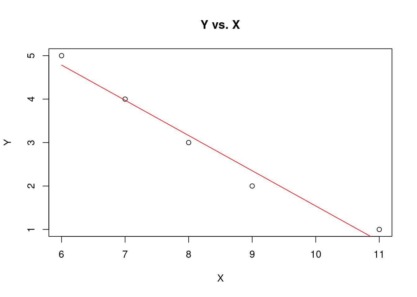
Find a straight line that best fits the following data:
\[ \begin{array}{c|cccccccccccc} x & 6 & 7 & 8 & 9 & 11 \\ \hline y & 5 & 4 & 3 & 2 & 1 \end{array} \]
Solution
Let the straight line be given by the equation \(Y = a + bX\). To determine the values of \(a\) and \(b\) for this line, we use the normal equations:
\[ \begin{array}{cccccc} \displaystyle \sum_{i=1}^{n} y_i &=& na & + & \displaystyle b \sum_{i=1}^{n} x_i \\ \displaystyle \sum_{i=1}^{n} y_i x_i &=& \displaystyle a \sum_{i=1}^{n}x_i & + & \displaystyle b\sum_{i=1}^{n}x_i^{2} \end{array} \] can be written as
\[ \begin{array}{cccccc} \displaystyle \sum y & = & na & + & \displaystyle b \sum x \\ \displaystyle \sum yx & = & \displaystyle a \sum x & + & \displaystyle b \sum x^{2} \end{array} \]
We need to calculate \(\displaystyle \sum y\), \(\displaystyle \sum x\), \(\displaystyle \sum xy\), and \(\displaystyle \sum x^2\), which can be obtained from the following table:
\[ \begin{array}{ccccccccccccc} i & x & y & x^2 & xy \\ \hline 1 & 6 & 5 & 36 & 30 \\ 2 & 7 & 4 & 49 & 28 \\ 3 & 8 & 3 & 64 & 24 \\ 4 & 9 & 2 & 81 & 18 \\ 5 & 11 & 1 & 121 & 11 \\ \hline n =5& \displaystyle \sum x = 41 & \displaystyle \sum y = 15 & \displaystyle \sum x^2 = 351 & \displaystyle \sum xy = 111 \\ \hline \end{array} \]
By substituting the values of \(\displaystyle \sum y\), \(\displaystyle \sum x\), \(\displaystyle \sum xy\), and \(\displaystyle \sum x^2\) into the normal equations, we obtain:
\[ \begin{array}{cccccc} \displaystyle 15 & = & 5 a & + & 41 b & & (1)\\ \displaystyle 111 & = & 41 a & + & 351 b & & (2) \end{array} \]
Now we solve equations (1) and (2).
Multiplying equation (1) by 41 and equation (2) by 5, i.e.
\[ \begin{array}{cccccc} \displaystyle 15 & = & 5 a & + & 41 b & & \times \quad 41 \\ \displaystyle 111 & = & 41 a & + & 351 b & & \times \quad 5 \end{array} \]
we have \[ \begin{array}{cccccc} \displaystyle 615 & = & 205 a & + & 168 b && (3) \\ \displaystyle 555 & = & 205 a & + & 1755 b && (4) \end{array} \]
Subtracting (3) from (4), we obtain
\[ \begin{array}{ccllllc} \displaystyle & -60 & = & 74 b & & \\ \displaystyle \Rightarrow & b & = & -60/74 & =& -0.8108 \end{array} \]
By substituting the value of \(b\) in equation (2), we have \[ \begin{array}{cclllllllll} & 15 & = & 5a+41\times (-0.8108) \\ & 15 & = & 5a - 33.2428 \\ \Rightarrow & a & = & 9.6486 \end{array} \]
with these values for \(a\) and \(b\), the equation for the line of best fit is: \(Y=9.6486-0.8108 X\).
# Create a data frame to store the data
X <- c(6, 7, 8, 9, 11)
Y <- c(5, 4, 3, 2, 1)
data <- data.frame(X, Y)
data| X | Y |
|---|---|
| 6 | 5 |
| 7 | 4 |
| 8 | 3 |
| 9 | 2 |
| 11 | 1 |
# Create a scatterplot of Y versus X
plot(
  data$X,
  data$Y,
  main = "Y vs. X",
  xlab = "X",
  ylab = "Y"
  )

# Fit a linear regression model to the data
linear_model <- lm(Y ~ X, data = data)

# Summarize the linear regression model
summary(linear_model)
##
## Call:
## lm(formula = Y ~ X, data = data)
##
## Residuals:
## 1 2 3 4 5
## 0.21622 0.02703 -0.16216 -0.35135 0.27027
##
## Coefficients:
## Estimate Std. Error t value Pr(>|t|)
## (Intercept) 9.64865 0.65370 14.76 0.000675 ***
## X -0.81081 0.07802 -10.39 0.001901 **
## ---
## Signif. codes: 0 '***' 0.001 '**' 0.01 '*' 0.05 '.' 0.1 ' ' 1
##
## Residual standard error: 0.3002 on 3 degrees of freedom
## Multiple R-squared: 0.973, Adjusted R-squared: 0.964
## F-statistic: 108 on 1 and 3 DF, p-value: 0.001901# Calculate the predicted Y for a range of X
predicted_values <- predict(
linear_model,
newdata = data.frame(X = seq(min(X),
max(X),
length.out = 5)
)
)
# Plot the data points and the predicted Y values
plot(
data$X,
data$Y,
main = "Y vs. X",
xlab = "X",
ylab = "Y"
)
lines(seq(min(X),
max(X),
length.out = 5),
predicted_values, col = "red"
)
3 Example 3
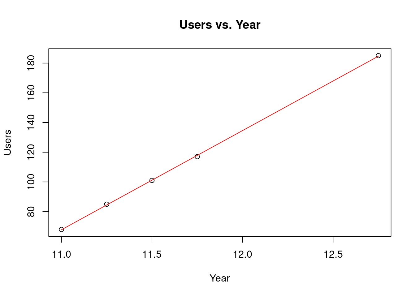
Find a straight line that best fits the following data:
\[ \begin{array}{c|c} \hline \textrm{Year} & \textrm{Twitter users} \\ \hline 11.00 & 68 \\ 11.25 & 85 \\ 11.50 & 101 \\ 11.75 & 117 \\ 12.75 & 185 \\ \hline \end{array} \]
Solution
Let the straight line be given by the equation \(Y = a + bX\). To determine the values of \(a\) and \(b\) for this line, we use the normal equations:
\[ \begin{array}{cccccc} \displaystyle \sum_{i=1}^{n} y_i &=& na & + & \displaystyle b \sum_{i=1}^{n} x_i \\ \displaystyle \sum_{i=1}^{n} y_i x_i &=& \displaystyle a \sum_{i=1}^{n}x_i & + & \displaystyle b\sum_{i=1}^{n}x_i^{2} \end{array} \]
can be written as
\[ \begin{array}{cccccc} \displaystyle \sum y & = & na &+& \displaystyle b \sum x \\ \displaystyle \sum yx & = & \displaystyle a \sum x &+& \displaystyle b \sum x^{2} \end{array} \] We need to calculate \(\displaystyle \sum y\), \(\displaystyle \sum x\), \(\displaystyle \sum xy\), and \(\displaystyle \sum x^2\), which can be obtained from the following table:
\[ \begin{array}{ccccccccccccc} i & x & y & x^2 & xy \\ \hline 1 & 11 & 68 & 121 & 748 \\ 2 & 11.25 & 85 & 126.5625 & 956.25 \\ 3 & 11.5 & 101 & 132.25 & 1161.5 \\ 4 & 11.75 & 117 & 138.0625 & 1374.75 \\ 5 & 12.75 & 185 & 162.5625 & 2358.75 \\ \hline n = 5& \displaystyle \sum x = 58.25 & \displaystyle \sum y = 556 & \displaystyle \sum x^2 = 680.4375 & \displaystyle \sum xy = 6599.25 \\ \hline \end{array} \]
By substituting the values of \(\displaystyle \sum y\), \(\displaystyle \sum x\), \(\displaystyle \sum xy\), and \(\displaystyle \sum x^2\) into the normal equations, we obtain:
\[ \begin{array}{cccccc} \displaystyle 556 & = & 5 a &+& 58.25 b && (1)\\ \displaystyle 6599.25 & = & 58.25 a &+& 680.4375 b & & (2) \end{array} \]
We will now solve equations (1) and (2) using Cramer’s rule. Let us proceed with the calculations:
\[ a = \dfrac{\det \left(\begin{array}{cc} 556 & 58.25 \\ 6599.25 & 680.4375 \end{array} \right)}{\det \left(\begin{array}{cc}5 & 58.25 \\ 58.25 & 680.4375 \end{array} \right)} = -666.6370\]
and
\[ b = \dfrac{\det \left(\begin{array}{cc} 5 & 556 \\ 58.25 & 6599.25 \end{array} \right)}{\det \left(\begin{array}{cc}5 & 58.25 \\ 58.25 & 680.4375 \end{array} \right)} = 66.7671\]
with these values for \(a\) and \(b\), the equation for the line of best fit is: \(Y=-666.6370+66.7671 X\).
# Create a data frame to store the data
Year <- c(11.00, 11.25, 11.50, 11.75, 12.75 )
Users <- c(68, 85, 101, 117, 185)
data <- data.frame(Year, Users)
data| Year | Users |
|---|---|
| 11.00 | 68 |
| 11.25 | 85 |
| 11.50 | 101 |
| 11.75 | 117 |
| 12.75 | 185 |
# Create a scatterplot of Y versus X
plot(
  data$Year,
  data$Users,
  main = "Users vs. Year",
  xlab = "Year",
  ylab = "Users"
  )

# Fit a linear regression model to the data
linear_model <- lm(Users~Year, data = data)

# Summarize the linear regression model
summary(linear_model)
##
## Call:
## lm(formula = Users ~ Year, data = data)
##
## Residuals:
## 1 2 3 4 5
## 0.1986 0.5068 -0.1849 -0.8767 0.3562
##
## Coefficients:
## Estimate Std. Error t value Pr(>|t|)
## (Intercept) -666.6370 5.5204 -120.8 1.25e-06 ***
## Year 66.7671 0.4732 141.1 7.85e-07 ***
## ---
## Signif. codes: 0 '***' 0.001 '**' 0.01 '*' 0.05 '.' 0.1 ' ' 1
##
## Residual standard error: 0.6393 on 3 degrees of freedom
## Multiple R-squared: 0.9998, Adjusted R-squared: 0.9998
## F-statistic: 1.991e+04 on 1 and 3 DF, p-value: 7.85e-07# Calculate the predicted Y for a range of X
predicted_values <- predict(
linear_model,
newdata = data.frame(Year = seq(min(Year),
max(Year),
length.out = 5)
)
)
# Plot the data points and the predicted Y values
plot(
data$Year,
data$Users,
main = "Users vs. Year",
xlab = "Year",
ylab = "Users"
)
lines(seq(min(Year),
max(Year),
length.out = 5),
predicted_values, col = "red"
)
3.1 Derivation of Cramer’s rule:
Let us start with:
\[\begin{align*} \displaystyle ax+by & =u \\ \displaystyle cx+dy & =v \end{align*}\]
Multiplying both sides of the first equation by \(c\) and both sides of the second equation by \(a\), then subtracting, we find that \[(ad−bc)y=av−uc.\] Assuming that the determinant \(ad−bc\) is not \(0\), we find that \[ y = \dfrac{av - uc}{ad - bc} = \dfrac{\det \left(\begin{array}{cc}a & u \\ c & v \end{array} \right)}{\det \left(\begin{array}{cc}a & b \\ c & d \end{array} \right)} = \dfrac{ \left|\begin{array}{cc}a & u \\ c & v \end{array} \right|}{ \left|\begin{array}{cc}a & b \\ c & d \end{array} \right|} \]
Multiplying both sides of the first equation by \(d\) and both sides of the second equation by \(b\), then subtracting, we find that \[(ad−bc)x=ud−vb.\] Assuming that the determinant \(ad−bc\) is not \(0\), we find that \[ x = \dfrac{ud−vb}{ad - bc} = \dfrac{\det \left(\begin{array}{cc}u & b \\ v & d \end{array} \right)}{\det \left(\begin{array}{cc}a & b \\ c & d \end{array} \right)} = \dfrac{ \left| \begin{array}{cc}u & b \\ v & d \end{array} \right|}{ \left|\begin{array}{cc}a & b \\ c & d \end{array} \right|}\]
4 Example 4
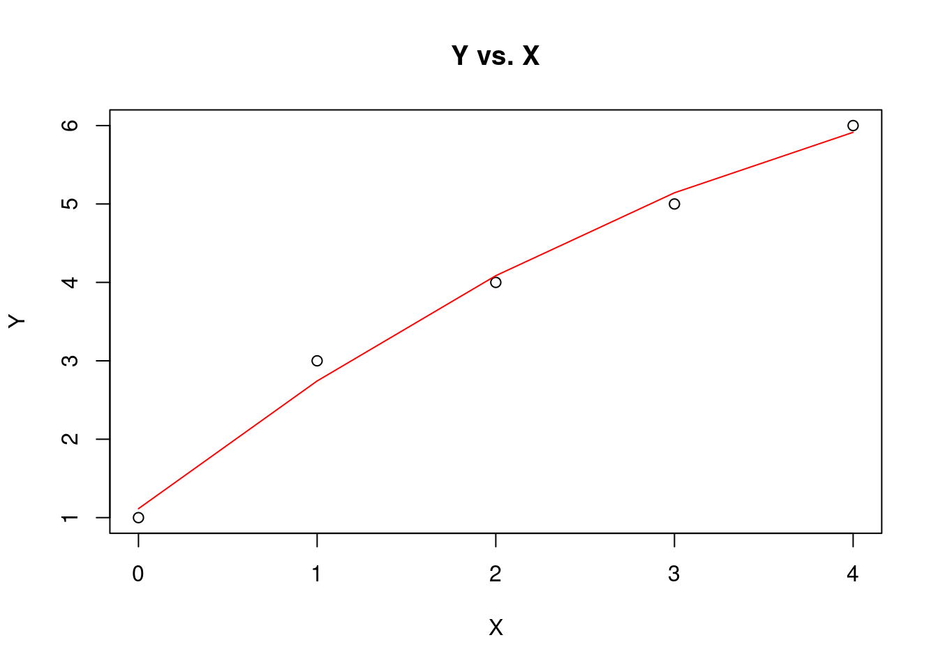
Fit a second-degree parabola to the following data:
\[ \begin{array}{c|cccccccccccc} x & y \\ \hline 0 & 1 \\ 1 & 3 \\ 2 & 4 \\ 3 & 5 \\ 4 & 6 \\ \hline \end{array} \]
Solution
Let \(Y = a+ bX + cX^2\) be the second-degree parabola, and we have to determine \(a\), \(b\) and \(c\). Normal equations for the second-degree parabola are
\[ \begin{array}{ccccccccccccc} \displaystyle \sum y & = & \displaystyle na & + & \displaystyle b \sum x & + & \displaystyle c \sum x^2 \\ \displaystyle \sum xy & = & \displaystyle a \sum x & + & \displaystyle b \sum x^2 & + & \displaystyle c \sum x^3 \\ \displaystyle \sum x^2y & = & \displaystyle a \sum x^2 & + & \displaystyle b \sum x^3 & + & \displaystyle c \sum x^4 \\ \end{array} \]
To solve the above normal equations, we need \(\displaystyle \sum y\), \(\displaystyle \sum x\), \(\displaystyle \sum xy\), \(\displaystyle \sum x^2 y\), \(\displaystyle \sum x^2\), \(\displaystyle \sum x^3\), and \(\displaystyle \sum x^4\), which are obtained from the following table:
\[ \begin{array}{ccccccccc} i & x & y & xy & x^2 & x^2y & x^3 & x^4 \\ \hline 1 & 0 & 1 & 0 & 0 & 0 & 0 & 0 \\ 2 & 1 & 3 & 3 & 1 & 3 & 1 & 1 \\ 3 & 2 & 4 & 8 & 4 & 16 & 8 & 16 \\ 4 & 3 & 5 & 15 & 9 & 45 & 27 & 81 \\ 5 & 4 & 6 & 24 & 16 & 96 & 64 & 256 \\ \hline n = 5& \displaystyle \sum x = 10 & \displaystyle \sum y = 19 & \displaystyle \sum xy = 50 & \displaystyle \sum x^2 = 30 & \displaystyle \sum x^2y = 160 & \displaystyle \sum x^3 = 100 & \displaystyle \sum x^4 = 354\\ \hline \end{array} \]
Substituting the values of \(\displaystyle \sum y\), \(\sum x\), \(\displaystyle \sum xy\), \(\displaystyle \sum x^2 y\), $x^2 $, \(\sum x^3\), and \(\displaystyle \sum x^4\) into the above normal equations, we have:
\[ \begin{array}{ccccccccccccc} \displaystyle \sum y & = & \displaystyle na & + & \displaystyle b \sum x & + & \displaystyle c \sum x^2 \\ \displaystyle \sum xy & = & \displaystyle a \sum x & + & \displaystyle b \sum x^2 & + & \displaystyle c \sum x^3 \\ \displaystyle \sum x^2y & = & \displaystyle a \sum x^2 & + & \displaystyle b \sum x^3 & + & \displaystyle c \sum x^4 \\ \end{array} \] \[ \begin{array}{ccccccccccccc} 19 & = & 5 a & + & 10 b & + & 30 c & & (1) \\ 50 & = & 10 a & + & 30 b & + & 100 c & & (2) \\ 160 & = & 30 a & + & 100 b & + & 354 c & & (3) \\ \end{array} \]
Now, we solve equations (1), (2) and (3).
Multiplying equation (1) by 2, we get
\[ \begin{array}{ccccccccccccc} 38 & = & 10 a &+& 20 b &+& 60 c && (4) \end{array} \]
Subtracting equation (4) from equation (2), we get
\[ \begin{array}{ccccccccccccc} 50 & = & 10 a & + & 30 b & + & 100 c & & (2) \\ 38 & = & 10 a & + & 20 b & + & 60 c & & (4) \\ \hline 12 & = & 0 a & + & 10 b & + & 40 c & & (5) \\ \end{array} \]
Multiplying equation (2) by 3, we get
\[ \begin{array}{ccccccccccccc} 150 & = & 30 a &+& 90 b &+& 300 c && (6) \end{array} \]
Subtracting equation (6) from equation (3), we get
\[ \begin{array}{ccccccccccccc} 160 & = & 30 a & + & 100 b & + & 354 c & & (3) \\ 150 & = & 30 a & + & 90 b & + & 300 c & & (6)\\ \hline 10 & = & 0 a & + & 10 b & + & 54 c & & (7) \\ \end{array} \]
Now we solve equation (5) and (7).
Subtracting equation (5) from equation (7), we get
\[ \begin{array}{ccccccccccccc} 12 & = & 0 a & + & 10 b & + & 40 c & & (5) \\ 10 & = & 0 a & + & 10 b & + & 54 c & & (7) \\ \hline 2 & = & & & 0 b & - & 14 c & & \\ \end{array} \]
\[ \begin{array}{cclllllllllllll} & 2 & = & - 14c \\ & c& = & -2/14 \\ \Rightarrow & c& = & -0.1429 \\ \end{array} \]
Substituting the value of \(\mathrm{c}\) in equation (7), we get
\[ \begin{array}{ccclllllllllll} & 10 & = & 10 b &+ & 54 (-0.1429 ) \\ & 10 & = & 10 b &- & 7.7166 \\ & 10 b & = & 10 &+ & 7.7166 \\ \Rightarrow & b & = & 1.77166 \\ \end{array} \]
Substituting the value of \(b\) and \(a\) in equation (1), we get
\[ \begin{array}{ccccccccccccc} & 19 & = & 5 a & + & 10 (1.77166) & + & 30 (-0.1429) \\ & 19 & = & 5 a & + & 17.717 & - & 4.287 \\ \Rightarrow & a & = & 1.114 \end{array} \]
Thus, the second degree of parabola of best fit is
\[Y=1.114+1.7717 X-0.1429 X^{2} \]
# Create a data frame to store the data
X <- c(0, 1, 2, 3, 4)
Y <- c(1, 3 ,4, 5, 6)
data <- data.frame(X, Y)
data| X | Y |
|---|---|
| 0 | 1 |
| 1 | 3 |
| 2 | 4 |
| 3 | 5 |
| 4 | 6 |
# Create a scatterplot of Y versus X
plot(
  data$X,
  data$Y,
  main = "Y vs. X",
  xlab = "X",
  ylab = "Y"
  )

# Fit a quadratic regression model to the data
quadratic_model <- lm(Y ~ X + I(X^2), data = data)

# Summarize the quadratic regression model
summary(quadratic_model)
##
## Call:
## lm(formula = Y ~ X + I(X^2), data = data)
##
## Residuals:
## 1 2 3 4 5
## -0.11429 0.25714 -0.08571 -0.14286 0.08571
##
## Coefficients:
## Estimate Std. Error t value Pr(>|t|)
## (Intercept) 1.11429 0.22497 4.953 0.0384 *
## X 1.77143 0.26650 6.647 0.0219 *
## I(X^2) -0.14286 0.06389 -2.236 0.1548
## ---
## Signif. codes: 0 '***' 0.001 '**' 0.01 '*' 0.05 '.' 0.1 ' ' 1
##
## Residual standard error: 0.239 on 2 degrees of freedom
## Multiple R-squared: 0.9923, Adjusted R-squared: 0.9846
## F-statistic: 128.5 on 2 and 2 DF, p-value: 0.007722# Calculate the predicted Y for a range of X
predicted_values <- predict(
quadratic_model,
newdata = data.frame(X = seq(min(X),
max(X),
length.out = 5)
)
)
# Plot the data points and the predicted Y values
plot(
data$X,
data$Y,
main = "Y vs. X",
xlab = "X",
ylab = "Y"
)
lines(seq(min(X),
max(X),
length.out = 5),
predicted_values, col = "red"
)
5 Example 5
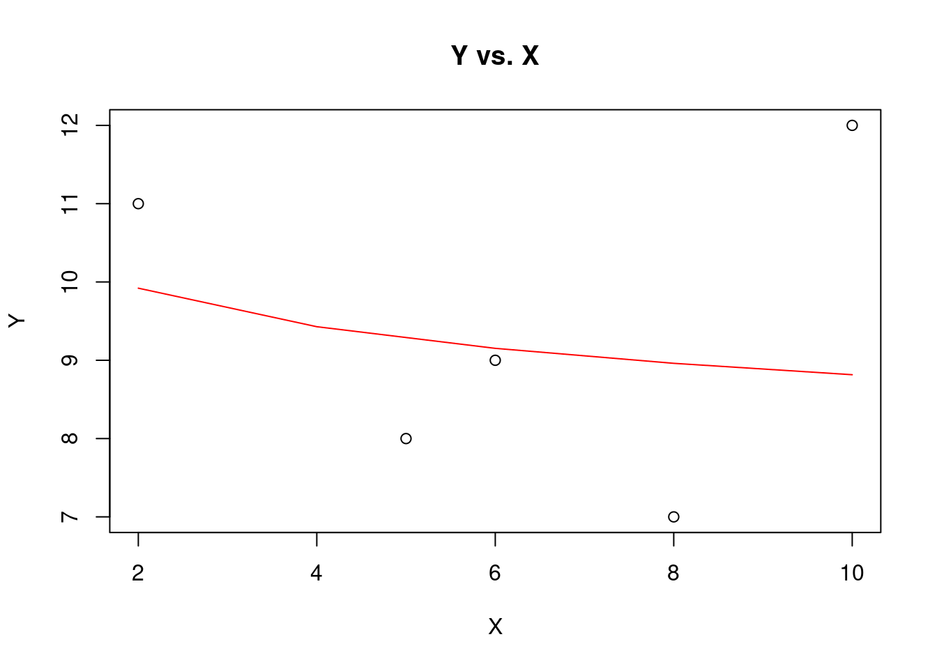
Fit the power curve \(Y = a X^b\) to the following data:
\[ \begin{array}{c|cccccccccccc} x & y \\ \hline 6 & 9 \\ 2 & 11 \\ 10 & 12 \\ 5 & 8 \\ 8 & 7 \\ \hline \end{array} \]
Solution
Let the power curve be \(Y=aX^b\), and the normal equations for estimating \(a\) and \(b\) are:
\[ \begin{array}{ccccccccccccc} \displaystyle \sum u & = & n A & + & \displaystyle b\sum v \\ \displaystyle \sum uv & = & \displaystyle A \sum v & + & \displaystyle b \sum v^{2} \end{array} \]
where \(u=\log y, v= \log x\), and \(A=\log a\).
Note: Here we are using \(\log\) with base \(10\).
To find the values of \(a\) and \(b\) from the above normal equations, we require \(\displaystyle \sum u\), \(\displaystyle \sum v\), \(\displaystyle \sum uv\), and \(\displaystyle \sum v^2\), which are calculated in the following table:
\[ \begin{array}{ccccccccc} i & x & y & u=\log y & v=\log x & uv & v^2 \\ \hline 1 & 6 & 9 & 0.954242509 & 0.77815125 & 0.742545002 & 0.605519368 \\ 2 & 2 & 11 & 1.041392685 & 0.301029996 & 0.313490435 & 0.090619058 \\ 3 & 10 & 12 & 1.079181246 & 1 & 1.079181246 & 1 \\ 4 & 5 & 8 & 0.903089987 & 0.698970004 & 0.631232812 & 0.488559067 \\ 5 & 8 & 7 & 0.84509804 & 0.903089987 & 0.763199578 & 0.815571525 \\ \hline n = 5& \displaystyle \sum x = 31 & \displaystyle \sum y = 47 & \displaystyle \sum u = 4.823004468 & \displaystyle \sum v= 3.681241237 & \displaystyle \sum uv = 3.529649074 & \displaystyle \sum v^2 = 3.000269018 \\ \hline \end{array} \]
Substituting the values \(\displaystyle \sum u=4.8230, \displaystyle \sum v =3.6812, \displaystyle \sum uv =3.5296\) and \(\displaystyle \sum v^{2}=3.0003\) into the above normal equations, we obtain:
\[ \begin{array}{ccccccccccccc} 4.8230 & = & 5 A & + & 3.6812 b & & (1) \\ 3.5296 & = & 3.6812 A & + & 3.0003 b & & (2) \end{array} \]
Now, we solve the equation (1) and equation (2).
Multiplying equation (1) by \(3.6812\) and equation (3) by \(5\), i.e.,
\[ \begin{array}{cccllllllllllc} 4.8230 & = 5 A & + & 3.6812 b && (1) \times 3.6812 \\ 3.5296 & = 3.6812 A & + & 3.0003 b && (2) \times 5 \end{array} \]
we have
\[ \begin{array}{ccccccccccccc} 17.7544 & = & 18.4060 A & + & 13.5512 b & & (3) \\ 17.6480 & = & 18.4060 A & + & 15.0015 b & & (4) \end{array} \]
Subtracting equation (4) from equation (3), we have
\[ \begin{array}{ccccccccccccc} & 0.1064 & = & -1.4503 b \\ \Rightarrow & b & = & -0.0734 \end{array} \]
Substituting the value of \(b\) in equation (1), we get
\[ \begin{array}{ccccccccccccc} 4.8230 & = & 5 A & + & 3.6812 (-0.0734) \\ A & = & 1.0186 \end{array} \]
Now \[a = \log^{-1} A= \log^{-1} (1.0186) = 10^{1.0186} = 10.4376\]
Thus, the power curve of the best fit is \(Y=10.4376 X^{-0.0734}.\)
| X | Y |
|---|---|
| 6 | 9 |
| 2 | 11 |
| 10 | 12 |
| 5 | 8 |
| 8 | 7 |
# Create a scatterplot of Y versus X
plot(
  data$X,
  data$Y,
  main = "Y vs. X",
  xlab = "X",
  ylab = "Y"
)

# Fit a quadratic regression model to the data
model <- lm(log10(Y) ~ log10(X), data = data)

# Summarize the quadratic regression model
summary(model)
##
## Call:
## lm(formula = log10(Y) ~ log10(X), data = data)
##
## Residuals:
## 1 2 3 4 5
## -0.007283 0.044852 0.133936 -0.064247 -0.107259
##
## Coefficients:
## Estimate Std. Error t value Pr(>|t|)
## (Intercept) 1.01863 0.15679 6.497 0.0074 **
## log10(X) -0.07339 0.20240 -0.363 0.7410
## ---
## Signif. codes: 0 '***' 0.001 '**' 0.01 '*' 0.05 '.' 0.1 ' ' 1
##
## Residual standard error: 0.109 on 3 degrees of freedom
## Multiple R-squared: 0.04198, Adjusted R-squared: -0.2774
## F-statistic: 0.1315 on 1 and 3 DF, p-value: 0.741# Calculate the value of a
a <- 10^((coef(model)[1]))
# Calculate the value of b
b <- coef(model)[2]
# Calculate the predicted Y for a range of X
predicted_values <- a*(seq(min(data$X), max(data$X), length.out = 5))^b
print(a)## (Intercept)
## 10.43836## log10(X)
## -0.07338735# Plot the data points and the predicted Y values
plot(
data$X,
data$Y,
main = "Y vs. X",
xlab = "X",
ylab = "Y"
)
lines(seq(min(data$X),
max(data$X),
length.out = 5),
predicted_values, col = "red"
)
6 Example 6
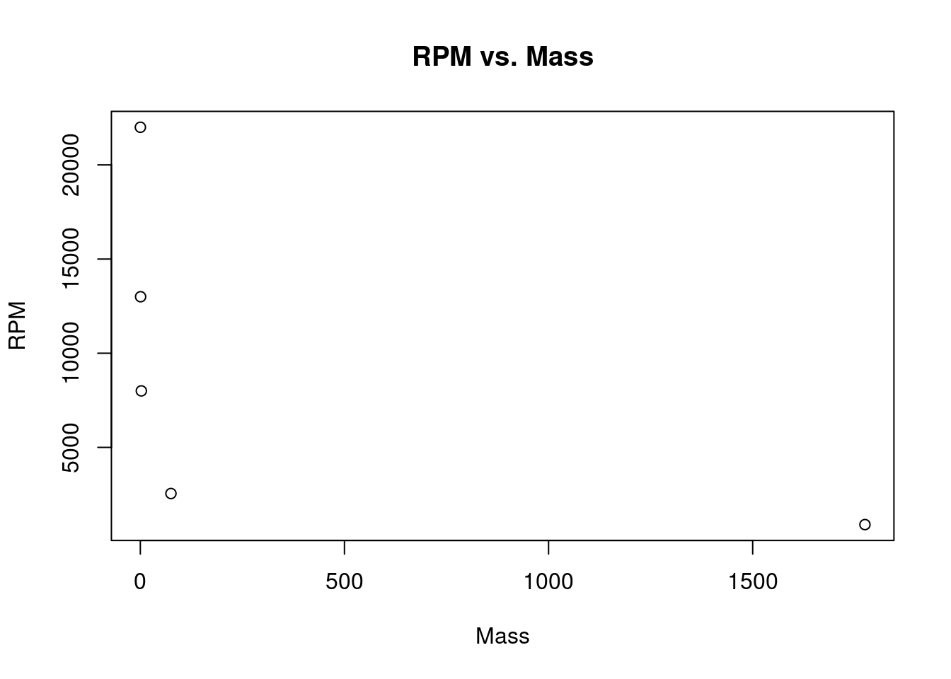
Fit the power curve \(Y = a X^b\) to the following data:
\[ \begin{array}{c|cccccccccccc} x & y \\ \hline 0.135 & 22000 \\ 0.67 & 13000 \\ 2.45 & 8000 \\ 75 & 2550 \\ 1775 & 900 \\ \hline \end{array} \]
Solution
Let the power curve be \(Y=aX^b\), and the normal equations for estimating \(a\) and \(b\) are:
\[ \begin{array}{ccccccccccccc} \displaystyle \sum u & = & n A & + & \displaystyle b\sum v \\ \displaystyle \sum uv & = & \displaystyle A \sum v & + & \displaystyle b \sum v^{2} \end{array} \]
where \(u=\log y, v= \log x\), and \(A=\log a\).
Note: Here we are using \(\log\) with base 10.
To find the values of \(a\) and \(b\) from the above normal equations, we require \(\displaystyle \sum u\), \(\displaystyle \sum v\), \(\displaystyle \sum uv\), and \(\displaystyle \sum v^2\), which are calculated in the following table:
\[ \begin{array}{ccccccccc} i & x & y & u=\log y & v=\log x & uv & v^2 \\ \hline 1 & 0.135 & 22000 & 4.342422681 & -0.869666232 & -3.776458368 & 0.756319354 \\ 2 & 0.67 & 13000 & 4.113943352 & -0.173925197 & -0.715518409 & 0.030249974 \\ 3 & 2.45 & 8000 & 3.903089987 & 0.389166084 & 1.518950247 & 0.151450241 \\ 4 & 75 & 2550 & 3.40654018 & 1.875061263 & 6.387471535 & 3.515854741 \\ 5 & 1775 & 900 & 2.954242509 & 3.249198357 & 9.598919909 & 10.55728997 \\ \hline n = 5& \displaystyle \sum x = 1853.255 & \displaystyle \sum y = 46450 & \displaystyle \sum u = 18.72023871 & \displaystyle \sum v= 4.469834276 & \displaystyle \sum uv = 13.01336491 & \displaystyle \sum v^2 = 15.01116428 \\ \hline \end{array} \]
Substituting the values of \(\displaystyle \sum u=18.72023871, \displaystyle \sum v=4.469834276,\sum uv= 13.01336491\) and \(\displaystyle \sum v^2=15.01116428\) into the above normal equations, we obtain:
\[ \begin{array}{ccccccccccccc} 1853.255 & = & 5 A & + & 4.469834276 b & & (1) \\ 13.01336491 & = & 4.469834276 A & + & 15.01116428 b & & (2) \end{array} \]
These two equations can be solved for \(A\) and \(b\) using Cramer’s rule:
\[A = \dfrac{\left| \begin{array}{cc} \color{red}{ \sum u} & \sum v \\ \color{red}{\sum uv} & \sum v^{2} \end{array} \right|} {\left| \begin{array}{cc} n & \sum v \\ \sum v & \sum v^{2} \end{array} \right|} = \dfrac{\left| \begin{array}{cc} \color{red}{18.72023871} & 4.469834276 \\ \color{red}{13.01336491} & 15.01116428 \end{array} \right|} {\left| \begin{array}{cc} 5 & 4.469834276\\ 4.469834276 & 15.01116428 \end{array} \right|} = 4.0461 \]
Now \(a = \log^{-1} (A) = \log^{-1} (4.0461) =10^{4.0461} = 11120\) and
\[b = \dfrac{\left| \begin{array}{cc} 5 & \color{red}{18.72023871} \\ 4.469834276 & \color{red}{13.01336491} \end{array} \right|} {\left| \begin{array}{cc} 5 & 4.469834276\\ 4.469834276 & 15.01116428 \end{array} \right|} = -0.3379 \]
Thus, the power curve of the best fit is \(Y=11120 X^{-0.3379}.\)
# Create a data frame to store the data
Mass <- c(0.135, 0.67, 2.45, 75, 1775)
RPM <- c(22000, 13000, 8000, 2550, 900)
data <- data.frame(Mass, RPM)
data| Mass | RPM |
|---|---|
| 0.135 | 22000 |
| 0.670 | 13000 |
| 2.450 | 8000 |
| 75.000 | 2550 |
| 1775.000 | 900 |
# Fit a power regression model to the data
power_model <- lm(log10(RPM) ~ log10(Mass), data = data)

# Summarize the power regression model
summary(power_model)
##
## Call:
## lm(formula = log10(RPM) ~ log10(Mass), data = data)
##
## Residuals:
## 1 2 3 4 5
## 0.002468 0.009070 -0.011523 -0.006010 0.005994
##
## Coefficients:
## Estimate Std. Error t value Pr(>|t|)
## (Intercept) 4.046107 0.005161 784.0 4.58e-09 ***
## log10(Mass) -0.337886 0.002979 -113.4 1.51e-06 ***
## ---
## Signif. codes: 0 '***' 0.001 '**' 0.01 '*' 0.05 '.' 0.1 ' ' 1
##
## Residual standard error: 0.009886 on 3 degrees of freedom
## Multiple R-squared: 0.9998, Adjusted R-squared: 0.9997
## F-statistic: 1.287e+04 on 1 and 3 DF, p-value: 1.51e-06# Calculate the value of a
a <- 10^((coef(model)[1]))
# Calculate the value of b
b <- coef(model)[2]
# Calculate the predicted Y for a range of X
predicted_values <- a*(seq(min(data$Mass), max(data$Mass), length.out = 5))^b
print(predicted_values)## [1] 12.090791 6.673574 6.342661 6.156732 6.028124## (Intercept)
## 10.43836## log10(X)
## -0.07338735# Plot the data points and the predicted Y values
plot(
data$Mass,
data$RPM,
main = "RPM vs. Mass",
xlab = "Mass",
ylab = "RPM"
)
lines(seq(min(data$Mass),
max(data$Mass),
length.out = 5),
predicted_values, col = "red"
)
7 Example 7
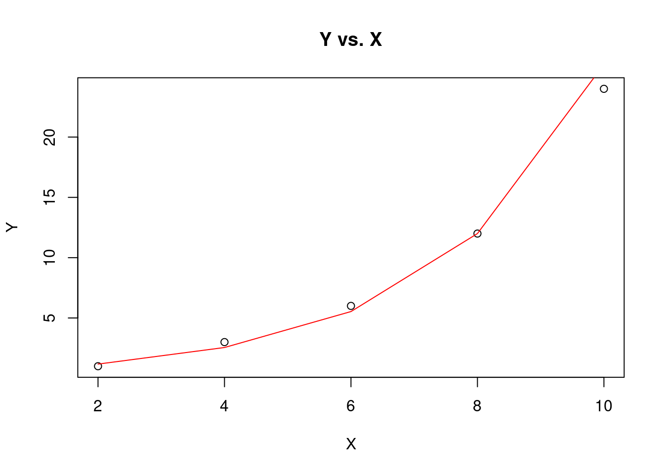
Fit the exponential curve \(Y=ab^X\) to the following data:
\[ \begin{array}{c|cccccccccccc} x & y \\ \hline 2 & 1 \\ 4 & 3 \\ 6 & 6 \\ 8 & 12 \\ 10 & 24 \\ \hline \end{array} \]
Solution
Let the exponential curve be \(Y=ab^X\), and the normal equations for estimating \(a\) and \(b\) are
\[ \begin{array}{ccccccccccccc} \displaystyle \sum u & = & n A & + & \displaystyle B \sum x \\ \displaystyle \sum ux & = & \displaystyle A \sum x & + & \displaystyle B \sum x^{2} \end{array} \]
where \(a=\log^{-1}(A)= 10^{A}\) and \(b= \log^{-1}(B)=10^{B}\).
Note: Here we are using \(\log\) with base \(10\).
To find the values of \(a\) and \(b\) from the above normal equations, we require \(\displaystyle \sum u\), \(\displaystyle \sum x, \displaystyle \sum ux\) and \(\displaystyle \sum x^{2}\), which are being calculated in the following table:
\[ \begin{array}{ccccccccc} i & x & y & u=\log y & ux & x^2 \\ \hline 1 & 2 & 1 & 0 & 0 & 4 \\ 2 & 4 & 3 & 0.477121255 & 1.908485019 & 16 \\ 3 & 6 & 6 & 0.77815125 & 4.668907502 & 36 \\ 4 & 8 & 12 & 1.079181246 & 8.633449968 & 64 \\ 5 & 10 & 24 & 1.380211242 & 13.80211242 & 100 \\ \hline n = 5& \displaystyle \sum x = 30 & \displaystyle \sum y = 46 & \displaystyle \sum u = 3.714664993 & \displaystyle \sum ux = 29.01295495 & \displaystyle \sum x^2 = 220 \\ \hline \end{array} \]
Substituting the values of \(\displaystyle \sum u , \displaystyle \sum x, \sum ux\) and \(\displaystyle \sum x^{2}\) in the above normal equations, we get
\[ \begin{array}{ccccccccccccc} 3.7147 & = & 5 A & + & 30 B & & (1) \\ 29.013 & = & 30 A & + & 220 B & & (2) \end{array} \]
Now, we solve the equation (1) and equation (2).
Multiplying equation (1) by \(6\), i.e.,
\[ \begin{array}{ccccccccccccc} 3.7147 & = & 5 A &+& 30 B & & (1) \times 6 \\ \end{array} \]
we have
\[ \begin{array}{ccccccccccccc} 22.2882 & = & 30 A & + & 180 B & & (3) \\ 29.013 & = & 30 A & + & 220 B & & (2) \end{array} \]
Subtracting equation (2) from equation (3), we have
\[ \begin{array}{ccccccccccccc} & 6.7248 & = & 40 B \\ \Rightarrow & B & = & 0.1681 \end{array} \]
Substituting the value of \(B\) in equation (1), we get
\[A=-0.26566\]
Now \[a = \log^{-1} A= \log^{-1} (-0.26566) = 10^{-0.26566} = 0.5424\]
and
\[b = \log^{-1} B= \log^{-1} (0.1681) = 10^{0.1681} = 1.4727\]
Thus, the exponential curve of the best fit is \(Y=0.5424(1.4727)^{X}.\)
| X | Y |
|---|---|
| 2 | 1 |
| 4 | 3 |
| 6 | 6 |
| 8 | 12 |
| 10 | 24 |
# Create a scatterplot of Y versus X
plot(
  data$X,
  data$Y,
  main = "Y vs. X",
  xlab = "X",
  ylab = "Y"
)

# Fit a quadratic regression model to the data
model <- lm(log10(Y) ~ X , data = data)

# Summarize the quadratic regression model
summary(model)
##
## Call:
## lm(formula = log10(Y) ~ X, data = data)
##
## Residuals:
## 1 2 3 4 5
## -7.044e-02 7.044e-02 3.522e-02 3.469e-17 -3.522e-02
##
## Coefficients:
## Estimate Std. Error t value Pr(>|t|)
## (Intercept) -0.26581 0.06744 -3.942 0.029106 *
## X 0.16812 0.01017 16.537 0.000481 ***
## ---
## Signif. codes: 0 '***' 0.001 '**' 0.01 '*' 0.05 '.' 0.1 ' ' 1
##
## Residual standard error: 0.0643 on 3 degrees of freedom
## Multiple R-squared: 0.9891, Adjusted R-squared: 0.9855
## F-statistic: 273.5 on 1 and 3 DF, p-value: 0.0004813# Calculate the value of a
a <- 10^((coef(model)[1]))
# Calculate the value of b
b <- 10^(coef(model)[2])
# Calculate the predicted Y for a range of X
predicted_values <- a*b^(seq(min(data$X), max(data$X), length.out = 5))
print(predicted_values)## [1] 1.176079 2.550849 5.532647 12.000000 26.027323## (Intercept)
## 0.5422359## X
## 1.472733# Plot the data points and the predicted Y values
plot(
data$X,
data$Y,
main = "Y vs. X",
xlab = "X",
ylab = "Y"
)
lines(seq(min(data$X),
max(data$X),
length.out = 5),
predicted_values, col = "red"
)
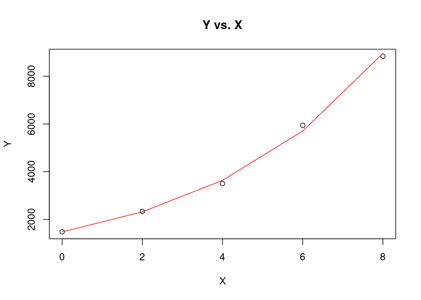
8 Example 8
Fit an exponential curve \(Y = a e^{bX}\) to the following data:
\[ \begin{array}{c|cccccccccccc} x & y \\ \hline 0 & 1481.66 \\ 2 & 2333.32 \\ 4 & 3501.39 \\ 6 & 5938.71 \\ 8 & 8838.60 \\ \hline \end{array} \]
Solution
Let the exponential curve be \(Y=a e^{bX}\), and the normal equations for estimating \(a\) and \(b\) are
\[ \begin{array}{ccccccccccccc} \displaystyle \sum u & = & n A & + & \displaystyle B \sum x \\ \displaystyle \sum ux & = & \displaystyle A \sum x & + & \displaystyle B \sum x^{2} \end{array} \]
where \(a=\log^{-1}(A)\) and \(b= \dfrac{B}{\log e}\).
Note: Here we are using \(\log\) with base \(10\).
To find the values of \(a\) and \(b\) from the above normal equations, we require \(\displaystyle \sum u, \sum x, \displaystyle \sum ux\) and \(\displaystyle \sum x^{2}\), which are being calculated in the following table:
\[ \begin{array}{ccccccccc} i & x & y & u=\log y & ux & x^2 \\ \hline 1 & 0 & 1481.66 & 3.170748557 & 0 & 0 \\ 2 & 2 & 2333.32 & 3.367974304 & 6.735948607 & 4 \\ 3 & 4 & 3501.39 & 3.544240487 & 14.17696195 & 16 \\ 4 & 6 & 5938.71 & 3.773692118 & 22.64215271 & 36 \\ 5 & 8 & 8838.6 & 3.94638348 & 31.57106784 & 64 \\ \hline n=5 & \displaystyle \sum x = 20 & \displaystyle \sum y = 22093.68 & \displaystyle \sum u = 17.80303895 & \displaystyle \sum ux = 75.1261311 & \displaystyle \sum x^2 = 120 \\ \hline \end{array} \]
Substituting the values of \(\displaystyle \sum u , \sum x , \sum ux\) and \(\displaystyle \sum x^{2}\) in the above normal equations, we get
\[ \begin{array}{ccccccccccccc} 17.80303895 & = & 5 A & + & 20 B & (1) \\ 75.1261311 & = & 20 A & + & 120 B & (2) \end{array} \]
By solving these equations as simultaneous equations, we get
\[ \begin{array}{ccccccccccccc} A & =& 3.1692 \\ B & = & 0.09784 \end{array} \]
Now \[a = \log^{-1} A= \log^{-1} (3.1692) = 10^{3.1692} = 1476.4\]
and
\[b = \dfrac{0.09784}{\log 2.71828} = \dfrac{0.09784}{0.43429} = 0.2253\]
Thus, the exponential curve of the best fit is \(Y=1476.4 \cdot e^{0.2253X}.\)
# Create a data frame to store the data
data <- data.frame(
  X = c(0, 2, 4, 6, 8),
  Y = c(1481.66, 2333.32, 3501.39, 5938.71, 8838.60)
)
data| X | Y |
|---|---|
| 0 | 1481.66 |
| 2 | 2333.32 |
| 4 | 3501.39 |
| 6 | 5938.71 |
| 8 | 8838.60 |
# Create a scatterplot of Y versus X
plot(
  data$X,
  data$Y,
  main = "Y vs. X",
  xlab = "X",
  ylab = "Y"
)

# Fit a quadratic regression model to the data
model <- lm(log(Y) ~ X , data = data)

# Summarize the quadratic regression model
summary(model)
##
## Call:
## lm(formula = log(Y) ~ X, data = data)
##
## Residuals:
## 1 2 3 4 5
## 0.003542 0.007058 -0.037687 0.040032 -0.012945
##
## Coefficients:
## Estimate Std. Error t value Pr(>|t|)
## (Intercept) 7.297376 0.025506 286.10 9.42e-08 ***
## X 0.225307 0.005206 43.27 2.72e-05 ***
## ---
## Signif. codes: 0 '***' 0.001 '**' 0.01 '*' 0.05 '.' 0.1 ' ' 1
##
## Residual standard error: 0.03293 on 3 degrees of freedom
## Multiple R-squared: 0.9984, Adjusted R-squared: 0.9979
## F-statistic: 1873 on 1 and 3 DF, p-value: 2.716e-05# Calculate the value of a
a <- exp(coef(model)[1])
# Calculate the value of b
b <- coef(model)[2]
# Calculate the predicted Y for a range of X
predicted_values <- a*exp(seq(min(data$X), max(data$X), length.out = 5)*b)
print(predicted_values)## [1] 1476.421 2316.909 3635.865 5705.669 8953.757## (Intercept)
## 1476.421## X
## 0.2253065# Plot the data points and the predicted Y values
plot(
data$X,
data$Y,
main = "Y vs. X",
xlab = "X",
ylab = "Y"
)
lines(seq(min(data$X),
max(data$X),
length.out = 5),
predicted_values, col = "red"
)
9 Exercise
9.1 Question 1
Consider the following data set: \[ \begin{array}{c|cccccccccccc} x & y \\ \hline 2 & 1 \\ 4 & 2 \\ 6 & 3 \\ 8 & 4 \\ 10 & 5 \\ \hline \end{array} \]
9.2 Question 2
Consider fit the power curve \(Y = a X^b\) to the following data: \[ \begin{array}{c|cccccccccccc} x & y \\ \hline 5 & 2 \\ 6 & 5 \\ 9 & 8 \\ 8 & 11 \\ 11 & 15 \\ \hline \end{array} \]
9.3 Question 3
Consider fit the power curve \(Y = ab^X\) to the following data: \[ \begin{array}{c|cccccccccccc} x & y \\ \hline 1 & 8 \\ 2 & 15 \\ 3 & 33 \\ 4 & 65 \\ 5 & 130 \\ \hline \end{array} \]
9.4 Question 4
Consider fit the Exponential curve \(Y = ae^{bX}\) to the following data: \[ \begin{array}{c|cccccccccccc} x & y \\ \hline 1 & 5 \\ 2 & 10 \\ 4 & 30 \\ \hline \end{array} \]
10 Solution
10.1 Question 1
Fit a second-degree parabola to the following data:
\[ \begin{array}{c|cccccccccccc} x & y \\ \hline 2 & 1 \\ 4 & 2 \\ 6 & 3 \\ 8 & 4 \\ 10 & 5 \\ \hline \end{array} \]
Let \(Y = a+ bX + cX^2\) be the second degree parabola and we have to determine \(a\), \(b\) and \(c\). The normal equations for the second-degree parabola are:
\[ \begin{array}{ccccccccccccc} \displaystyle \sum y & = & na & + & \displaystyle b \sum x & + & \displaystyle c \sum x^2 \\ \displaystyle \sum xy & = & \displaystyle a \sum x & + & \displaystyle b \sum x^2 & + & \displaystyle c \sum x^3 \\ \displaystyle \sum x^2y & = & \displaystyle a \sum x^2 & + & \displaystyle b \sum x^3 & + & \displaystyle c \sum x^4 \\ \end{array} \]
To solve above normal equations, we need \(\displaystyle \sum y,\) \(\displaystyle \sum x\), \(\displaystyle \sum xy,\) \(\displaystyle \sum x^2 y\), \(\displaystyle \sum x^2\), \(\displaystyle \sum x^3\) and \(\displaystyle \sum x^4\), which are obtained from following table:
\[ \begin{array}{ccccccccc} i & x & y & xy & x^2 & x^2y & x^3 & x^4 \\ \hline 1 & 2 & 1 & 2 & 4 & 4 & 8 & 16 \\ 2 & 4 & 2 & 8 & 16 & 32 & 64 & 256 \\ 3 & 6 & 3 & 18 & 36 & 108 & 216 & 1296 \\ 4 & 8 & 4 & 32 & 64 & 256 & 512 & 4096 \\ 5 & 10 & 5 & 50 & 100 & 500 & 1000 & 10000 \\ n = 5& \displaystyle \sum x = 30 & \displaystyle \sum y = 15 & \displaystyle \sum xy = 110 & \displaystyle \sum x^2 = 220 & \displaystyle \sum x^2y = 900 & \displaystyle \sum x^3 = 1800 & \displaystyle \sum x^4 = 15664 \\ \hline \end{array} \]
Substituting the values of \(\displaystyle \sum y, \sum x, \displaystyle \sum xy, \displaystyle \sum x^2 y, \displaystyle \sum x^2,\sum x^{3}\) and \(\displaystyle \sum x^{4}\) into the above normal equations, we have
\[ \begin{array}{ccccccccccccc} \displaystyle \sum y & = & na & + & \displaystyle b \sum x & + & \displaystyle c \sum x^2 \\ \displaystyle \sum xy & = & \displaystyle a \sum x & + & \displaystyle b \sum x^2 & + & \displaystyle c \sum x^3 \\ \displaystyle \sum x^2y & = & \displaystyle a \sum x^2 & + & \displaystyle b \sum x^3 & + & \displaystyle c \sum x^4 \\ \end{array} \]
\[ \begin{array}{ccccccccc} 15 & = & 5 a & + & 30 b & + & 220 c & & (1) \\ 110 & = & 30 a & + & 220 b & + & 1800 c & & (2) \\ 900 & = & 220 a & + & 1800 b & + & 15664 c & & (3) \\ \end{array} \]
The values of \(a\), \(b\) and \(c\) are obtained by solving equations using Cramer’s rule:
\[ a= \dfrac{\left| \begin{array}{cccc} \color{red}{\sum y} & \sum x & \sum x^{2} \\ \color{red}{\sum xy} & \sum x^{2} & \sum x^{3} \\ \color{red}{\sum x^{2}y} & \sum x^{3} & \sum x^{4} \end{array} \right|}{\left| \begin{array}{cccc} n & \sum x & \sum x^{2} \\ \sum x & \sum x^{2} & \sum x^{3} \\ \sum x^{2} & \sum x^{3} & \sum x^{4} \end{array} \right|} \]
\[ b= \dfrac{\left| \begin{array}{cccc} n & \color{red}{\sum y} & \sum x^{2} \\ \sum x & \color{red}{\sum xy} & \sum x^{3} \\ \sum x^{2} & \color{red}{\sum x^{2}y} & \sum x^{4} \end{array} \right|}{\left| \begin{array}{cccc} n & \sum x & \sum x^{2} \\ \sum x & \sum x^{2} & \sum x^{3} \\ \sum x^{2} & \sum x^{3} & \sum x^{4} \end{array} \right|} \] and \[ c= \dfrac{\left| \begin{array}{cccc} n & \sum x & \color{red}{\sum y} \\ \sum x & \sum x^{2} & \color{red}{\sum xy}\\ \sum x^{2} & \sum x^{3} & \color{red}{\sum x^{2}y} \end{array} \right|}{\left| \begin{array}{cccc} n & \sum x & \sum x^{2} \\ \sum x & \sum x^{2} & \sum x^{3} \\ \sum x^{2} & \sum x^{3} & \sum x^{4} \end{array} \right|} \] In order to further solve \(a\), \(b\) and \(c\), we need to know how to solve a three-by-three determinant.
Consider the determinant
\[ {\left| \begin{array}{cccc} a & b & c \\ d & e & f \\ g & h & i \end{array} \right|} \] The formula to solve a three-by-three determinant using the co-factor expansion is as follows:
\[ {\left| \begin{array}{cccc} a & b & c \\ d & e & f \\ g & h & i \end{array} \right|} = a \left| \begin{array}{cccc} e & f \\ h & i \end{array} \right| - b \left| \begin{array}{cccc} d & f \\ g & i \end{array} \right| + c \left| \begin{array}{cccc} d & e \\ g & h \end{array} \right| \]
With these values of \(a\), \(b\) and \(c\), the second degree parabola \(Y=a+bX+cX^{2}\) is the best fit.
\[ a = \dfrac{\left| \begin{array}{cccc} \color{red}{15} & 30 & 220 \\ \color{red}{110} & 220 & 1800 \\ \color{red}{900} & 1800 & 15664 \end{array} \right|}{\left| \begin{array}{cccc} 5 & 30 & 220 \\ 30 & 220 & 1800 \\ 220 & 1800 & 15664 \end{array} \right|} = 0 \\ \]
Now, we have \[ {\left| \begin{array}{cccc} \color{blue}{15} & \color{blue}{30} & \color{blue}{220} \\ 110 & 220 & 1800 \\ 900 & 1800 & 15664 \end{array} \right|} = \color{blue}{15} \left| \begin{array}{cccc} 220 & 1800 \\ 1800 & 15664 \end{array} \right| - \color{blue}{30} \left| \begin{array}{cccc} 110 & 1800 \\ 900 & 16554 \end{array} \right| + \color{blue}{220} \left| \begin{array}{cccc} 110 & 220 \\ 900 & 1800 \end{array} \right| = 0 \] and \[ {\left| \begin{array}{cccc} \color{blue}{5} & \color{blue}{30} & \color{blue}{220} \\ 30 & 220 & 1800 \\ 220 & 1800 & 15664 \end{array} \right|} =\color{blue}{5} \left| \begin{array}{cccc} 220 & 1800 \\ 1800 & 15664 \end{array} \right| - \color{blue}{30} \left| \begin{array}{cccc} 110 & 1800 \\ 990 & 16554 \end{array} \right| + \color{blue}{220} \left| \begin{array}{cccc} 110 & 220 \\ 900 & 1800 \end{array} \right| = 44800 \]
\[ b= \dfrac{\left| \begin{array}{cccc} 5 & \color{red}{15} & 220 \\ 30 & \color{red}{110} & 1800 \\ 220 & \color{red}{900} & 15664 \end{array} \right|}{\left| \begin{array}{cccc} 5 & 30 & 220 \\ 30 & 220 & 1800 \\ 220 & 1800 & 15664 \end{array} \right|} = \frac{1}{2} \] and \[ c= \dfrac{\left| \begin{array}{cccc} 5 & 30 & \color{red}{15} \\ 30 & 220 & \color{red}{110} \\ 220 & 1800 & \color{red}{990} \end{array} \right|}{\left| \begin{array}{cccc} 5 & 30 & 220 \\ 30 & 220 & 1800 \\ 220 & 1800 & 15664 \end{array} \right|} = 0 \]
Thus, the second degree of parabola of best fit is
\[Y= X/2 \]
10.1.1
A, B
10.1.2
Correct order: 1. Decide the model to fit in the dataset. 2. Find the corresponding summations for the normal function. 3. Using Cramer’s Rule to solve the linear system. 4. Find the determinent of each corresponding matrix and get the values of each coefficients.
10.1.3
0.5
10.1.4
0
10.2 Question 2
Fit the power curve \(Y = a X^b\) to the following data:
\[ \begin{array}{c|cccccccccccc} x & y \\ \hline 5 & 2 \\ 6 & 5 \\ 9 & 8 \\ 8 & 11 \\ 11 & 15 \\ \hline \end{array} \]
Let the power curve be \(Y=aX^b\), and the normal equations for estimating \(a\) and \(b\) are
\[ \begin{array}{ccccccccccccc} \displaystyle \sum u & = & n A & + & \displaystyle b\sum v \\ \displaystyle \sum uv & = & \displaystyle A \sum v & + & \displaystyle b \sum v^{2} \end{array} \]
where \(u=\log y, v= \log x\) and \(A=\log a\).
Note: Here we are using \(\log\) with base 10.
To find the values of \(a\) and \(b\) from the above normal equations, we require \(\displaystyle \sum u\) , \(\displaystyle \sum v, \displaystyle \sum uv\) and \(\displaystyle \sum v^{2}\) ,which are being calculated in the following table:
\[ \begin{array}{ccccccccc} i & x & y & u=\log y & v=\log x & uv & v^2 \\ \hline 1 & 5 & 2 & 0.301029996 & 0.698970004 & 0.210410937 & 0.488559067 \\ 2 & 6 & 5 & 0.698970004 & 0.77815125 & 0.543904383 & 0.605519368 \\ 3 & 9 & 8 & 0.903089987 & 0.954242509 & 0.861766855 & 0.910578767 \\ 4 & 8 & 11 & 1.041392685 & 0.903089987 & 0.940471306 & 0.815571525 \\ 5 & 11 & 15 & 1.176091259 & 1.041392685 & 1.224772834 & 1.084498725 \\ \hline n = 5& \displaystyle \sum x = 39 & \displaystyle \sum y = 41 & \displaystyle \sum u = 4.120573931 & \displaystyle \sum v= 4.375846436 & \displaystyle \sum uv = 3.781326316 & \displaystyle \sum v^2 = 3.904727452 \\ \hline \end{array} \]
Substituting the values of \(\displaystyle \sum u=4.1206, \displaystyle \sum v=4.3759,\sum uv=3.7814\) and \(\displaystyle \sum v^2=3.9048\) into the above normal equations, we obtain
\[ \begin{array}{ccccccccc} 4.1206 & = & 5 A & + & 4.3759 b & & (1) \\ 3.7184 & = & 4.3759 A & + & 3.9048 b & & (2) \end{array} \]
These two equations can be solved for \(a\) and \(b\) using Cramer’s rule:
\[A = \dfrac{\left| \begin{array}{cc} \color{red}{ \sum u} & \sum v \\ \color{red}{\sum uv} & \sum v^{2} \end{array} \right|} {\left| \begin{array}{cc} n & \sum v \\ \sum v & \sum v^{2} \end{array} \right|} = \dfrac{\left| \begin{array}{cc} \color{red}{4.1206} & 4.3759 \\ \color{red}{3.7184} & 3.9048 \end{array} \right|} {\left| \begin{array}{cc} 5 & 4.3759 \\ 4.3759 & 3.9048 \end{array} \right|} = −0.4571 \]
Now \(a = \log^{-1} (A) = \log^{-1} (−0.4571) = 10^{0.3491} = 0.3491\) and \[b = \dfrac{\left| \begin{array}{cc} 5 & \color{red}{4.3759} \\ 4.3759 & \color{red}{3.9048} \end{array} \right|} {\left| \begin{array}{cc} 5 & 4.3759 \\ 4.3759 & 3.9048 \end{array} \right|} = 1.4964 \]
Thus, the power curve of the best fit is \(Y=0.3491 X^{1.4964}.\)
10.2.1
C
10.2.2
A, C
10.2.3
3.905
10.2.4
0.0670
10.3 Question 3
Fit the power curve \(Y = a b^X\) to the following data:
\[ \begin{array}{c|cccccccccccc} x & y \\ \hline 1 & 8 \\ 2 & 15 \\ 3 & 33 \\ 4 & 65 \\ 5 & 130 \\ \hline \end{array} \]
Let the exponential curve be \(Y=ab^x\), and the normal equations for estimating \(a\) and \(b\) are
\[ \begin{array}{ccccccccccccc} \displaystyle \sum u & = & n A & + & \displaystyle B \sum x \\ \displaystyle \sum ux & = & \displaystyle A \sum x & + & \displaystyle B \sum x^{2} \end{array} \]
where \(a=\log^{-1}(A)\) and \(b= \log^{-1}(B)\).
Note: Here we are using \(\log\) with base 10.
To find the values of \(a\) and \(b\) from the above normal equations, we require \(\displaystyle \sum u\), \(\displaystyle \sum x, \displaystyle \sum ux\) and \(\displaystyle \sum x^{2}\), which are being calculated in the following table:
\[ \begin{array}{ccccccccc} i & x & y & u=\log y & ux & x^2 \\ \hline 1 & 1 & 8 & 0.903089987 & 0.903089987 & 1 \\ 2 & 2 & 15 & 1.176091259 & 2.352182518 & 4 \\ 3 & 3 & 33 & 1.51851394 & 4.55554182 & 9 \\ 4 & 4 & 65 & 1.812913357 & 7.251653427 & 16 \\ 5 & 5 & 130 & 2.113943352 & 10.56971676 & 25 \\ \hline n = 5 & \displaystyle \sum x = 15 & \displaystyle \sum y = 251 & \displaystyle \sum u = 7.524551895 & \displaystyle \sum ux = 25.63218451 & \displaystyle \sum x^2 = 55 \\ \hline \end{array} \]
Substituting the values of \(\displaystyle \sum u, \sum x, \sum ux\) and \(\displaystyle \sum x^{2}\) into the above normal equations, we get
\[ \begin{array}{ccccccccc} 7.5246 & = & 5 A & + & 15 B & & (1) \\ 25.6322 & = & 15 A & + & 55 B & & (2) \end{array} \]
Now, we solve the equation (1) and equation (2).
Multiplying equation (1) by \(3\), i.e.,
\[ \begin{array}{ccccccccc} 22.5738 & = & 15 A &+& 45 B && (1) \times 3 \\ \end{array} \]
we have
\[ \begin{array}{ccccccccc} 22.5738 & = & 15 A & +& 45 B && (3) \\ 25.6322 & = & 15 A &+& 55 B && (2) \end{array} \]
Subtracting equation (2) from equation (3), we have
\[ \begin{array}{ccccccccc} & 3.0584 & = & -10 B \\ \Rightarrow & B & = & -0.30584 \end{array} \]
Substituting the value of \(B\) in equation (1), we get
\[A=2.4224\]
Now \[a = \log^{-1} A= \log^{-1} (2.4224) = 10^{2.4224}=264.5087\]
and
\[b = \log^{-1} B= \log^{-1} (-0.30584) = 10^{-0.30584} = 0.4494\]
Thus, the exponential curve of the best fit is \(Y=264.5087 \cdot ( 0.4494 )^{X}.\)
10.3.1 3.1
C
10.3.2 3.2
A
10.3.3 3.3
80.8728
10.3.4 3.4
32811.38
10.4 Question 4
Fit an exponential curve \(Y = a e^{bX}\) to the following data:
\[ \begin{array}{c|cccccccccccc} x & y \\ \hline 1 & 5 \\ 2 & 10 \\ 4 & 30 \\ \hline \end{array} \]
Let the exponential curve be \(Y=a e^{bX}\), and the normal equations for estimating \(a\) and \(b\) are:
\[ \begin{array}{ccccccccccccc} \displaystyle \sum u & = & n A & + & \displaystyle B \sum x \\ \displaystyle \sum ux & = & \displaystyle A \sum x & + & \displaystyle B \sum x^{2} \end{array} \]
where \(a=\log^{-1}(A)\) and \(b= \dfrac{B}{\log e}\).
Note: Here we are using \(\log\) with base 10.
To find the values of \(a\) and \(b\) from the above normal equations, we require \(\displaystyle \sum u , \sum x\), \(\displaystyle \sum ux\) and \(\displaystyle \sum x^{2}\), which are being calculated in the following table:
\[ \begin{array}{ccccccccc} i & x & y & u=\log y & ux & x^2 \\ \hline 1 & 1 & 5 & 0.698970004 & 0.698970004 & 1 \\ 2 & 2 & 10 & 1 & 2 & 4 \\ 3 & 4 & 30 & 1.477121255 & 5.908485019 & 16 \\ \hline n= 3& \displaystyle \sum x = 7 & \displaystyle \sum y = 45 & \displaystyle \sum u = 3.176091259 & \displaystyle \sum ux = 8.607455023 & \displaystyle \sum x^2 = 21 \\ \hline \end{array} \]
Substituting the values of \(\displaystyle \sum u , \sum x , \sum ux\) and \(\displaystyle \sum x^{2}\) into the above normal equations, we get
\[ \begin{array}{ccccccccc} 3.1761 & = & 3 A & + & 7 B & & (1) \\ 8.6075 & = & 7 A & + & 21 B & & (2) \end{array} \]
By solving these equations as simultaneous equations, we get
\[ \begin{array}{ccccccccc} A & = & 0.4604 \\ B & = & 0.2564 \end{array} \]
Now \[a = \log^{-1} A= \log^{-1} (0.4604) = 10^{0.4604} = 2.8867\]
and
\[b = \dfrac{0.2564}{\log 2.71828} = \dfrac{0.2564}{0.43429} = 0.5904\]
Thus, the exponential curve of the best fit is \(Y=2.8867 \cdot e^{0.5904X}.\)
10.4.1
B
10.4.2
C
10.4.3
0.5904
10.4.4
0.7884