Overfitting and Underfitting with Polynomial Regression
1 Introduction
Overfitting poses a significant challenge for data scientists training supervised models.
It can severely impact performance and lead to dangerous outcomes in real-world applications.
But what exactly is overfitting?
過度擬合對於訓練監督模型的數據科學家來說是一個重大挑戰。
它會嚴重影響性能,並在現實應用中導致危險的結果。
但究竟什麼是過度擬合?
2 What is overfitting?
Overfitting occurs when a model learns too much from the training data and can’t apply the patterns to new data.
This means the model is very accurate with the training data but loses accuracy with new datasets.
過度擬合發生在模型從訓練數據中學習過多,無法將模式應用於新數據時。
這意味著模型在訓練數據上非常準確,但在新數據集上會失去準確性。
3 Why does it happen?
In machine learning, simplicity is important. We aim to generalize from training data, but complex models increase the risk of overfitting.
Complex models over-learn and mistake random errors for patterns, leading to overfitting.
Complexity is measured by the number of parameters, like in linear regression or neural networks.
Fewer parameters mean simpler models and lower risk of overfitting.
在機器學習中,簡單性很重要。我們的目標是從訓練數據中進行泛化,但複雜的模型會增加過度擬合的風險。
複雜的模型過度學習,並將隨機錯誤誤認為模式,導致過度擬合。
複雜性由參數的數量來衡量,例如在線性回歸或神經網絡中。
更少的參數意味著更簡單的模型和更低的過度擬合風險。
Here is a common data-fitting problem:
這是一個常見的數據擬合問題:
4 An example of overfitting
Let us create 21 points following the formula: \[ Y = - X^2 \]
Each point will have a normally distributed error with a mean of \(0\) and a standard deviation of \(0.05\). In real-life data science, data always has some random error.
After creating this dataset, we’ll fit polynomial models of increasing degrees and observe the results on both the training set and the test set. In real life, we don’t know the true model in our dataset, so we try different models to see which fits best.
We’ll use the first \(12\) points as the training set and the last \(9\) points as the test set.
Let’s now create the sample points:
讓我們按照公式創建21個點: \[ Y = - X^2 \]
每個點將具有均值為0且標準差為0.05的正態分佈誤差。在現實數據科學中,數據總是有一些隨機誤差。
創建此數據集後,我們將擬合逐漸增加次數的多項式模型,並觀察訓練集和測試集上的結果。在現實中,我們不知道數據集中的真實模型,所以我們嘗試不同的模型來看看哪個最合適。
我們將使用前12個點作為訓練集,最後9個點作為測試集。
現在讓我們創建樣本點:
# Load necessary libraries
library(ggplot2)

# Set seed for reproducibility
set.seed(0)

# Generate data
x <- seq(-1, 1, by = 0.1)
y <- -x^2 + rnorm(length(x), mean = 0, sd = 0.05)

# Create a data frame
data <- data.frame(x = x, y = y)

# Plot the data using ggplot2
ggplot(data, aes(x = x, y = y)) +
  geom_point(color = "blue", size = 3) +  # Scatter plot
  labs(x = "x", y = "y", title = "Scatter Plot of Generated Data") +
  theme_minimal()
As you can see, there’s some noise, just like in real-life fitting.
Let’s split this dataset into training and test sets using three different folds:
如你所見,有一些噪音,就像在現實中的擬合一樣。
讓我們使用三個不同的折疊將這個數據集分成訓練集和測試集:
\[ \begin{array}{cc|c} \textrm{Fold 1}&\color{blue}{\textrm{Training Data}} & \color{red}{\textrm{Test Data}} \\ \hline &1:12 & 13:21\\ \end{array} \] \[ \begin{array}{cc|c|c} \textrm{Fold 2}& \color{red}{\textrm{Test Data}} & \color{blue}{\textrm{Training Data}} & \color{red}{\textrm{Test Data}} \\ \hline & 1:4 & 5:16 & 17:21\\ \end{array} \]
\[ \begin{array}{cc|c} \textrm{Fold 3} &\color{red}{\textrm{Test Data}} & \color{blue}{\textrm{Training Data}} \\ \hline & 1:9 & 10:21\\ \end{array} \]
5 Performing the cross-validation calculations in Fold 1
Now, let’s split this dataset into training and test sets using Fold 1:
\[ \begin{array}{cc|c} \textrm{Fold 1}&\color{blue}{\textrm{Training Data}} & \color{red}{\textrm{Test Data}} \\ \hline &1:12 & 13:21\\ \end{array} \]
# Load necessary libraries
library(ggplot2)

# Set seed for reproducibility
set.seed(0)

# Generate data
x <- seq(-1, 1, by = 0.1)
y <- -x^2 + rnorm(length(x), mean = 0, sd = 0.05)

# Create a data frame
data <- data.frame(x = x, y = y)

# Split data into training and test sets
X_train <- data[1:12, ]
X_test <- data[13:nrow(data), ]

# Create a combined data frame for plotting
X_train$set <- "Training Set"
X_test$set <- "Test Set"
combined_data <- rbind(X_train, X_test)

# Plot the data using ggplot2
ggplot(combined_data, aes(x = x, y = y, color = set)) +
  geom_point(size = 3) +  # Scatter plot
  scale_color_manual(values = c("Training Set" = "blue", "Test Set" = "red")) +
  labs(x = "x", y = "y", title = "Scatter Plot of Generated Data") +
  theme_minimal()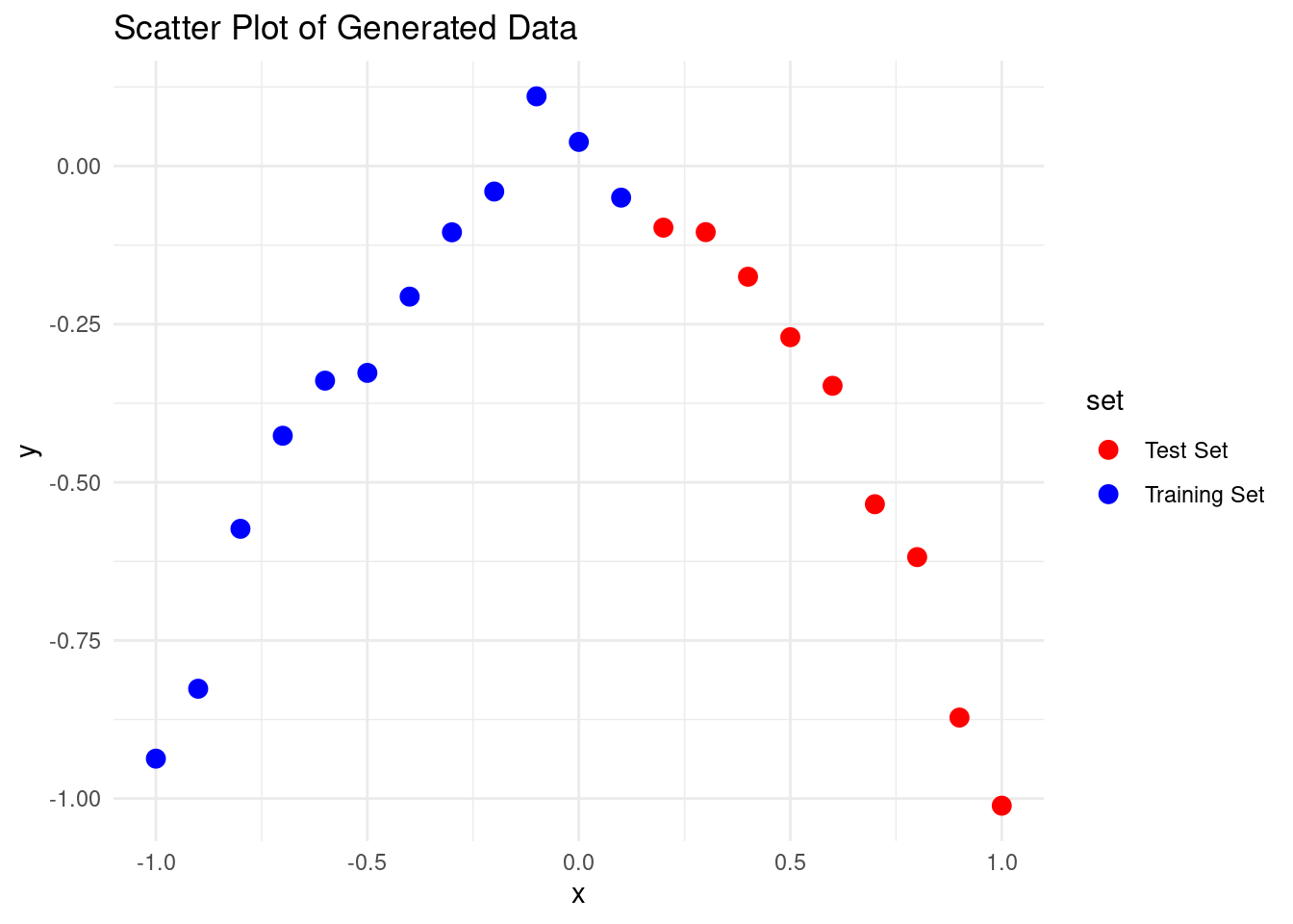
We can create a function that takes the training set and polynomial degree, and returns the best-fitting polynomial.
Polynomials are functions that have the form: \[ f(x) = a_n x^n + a_{n-1}x^{n-1} + \cdots + a_{0} \] The coefficients are real numbers, \(a_n, a_{n-1}, \cdots, a_1, a_0\) are real numbers, and \(n\), which is a nonnegative integer, is the degree, or order, of the polynomial.
Examples of polynomials are: \[ \begin{array}{lcccccccc} f(x) = 5x^5 + 6x^2 + 7x+ 3 && \textrm{polynomial of degree 5.} \\ f(x) = 2x^2 - 4x + 10 && \textrm{polynomial of degree 2.} \\ f(x) = 11x -3 && \textrm{polynomial of degree 1.} \end{array} \] A constant (e.g., \(f(x) = 6\)) is a polynomial of degree \(0\).
Then, we’ll make another function to plot the dataset and the best-fitting polynomial for a given degree.
Let’s start with a polynomial of degree \(1.\)
# Load necessary libraries
library(ggplot2)

# Set seed for reproducibility
set.seed(0)

# Generate data
x <- seq(-1, 1, by = 0.1)
y <- -x^2 + rnorm(length(x), mean = 0, sd = 0.05)

# Create a data frame
data <- data.frame(x = x, y = y)

# Split data into training and test sets
train_data <- data[1:12, ]
test_data <- data[13:nrow(data), ]

# Polynomial fit function
polynomial_fit <- function(degree = 1) {
  lm(y ~ poly(x, degree), data = train_data)
}

# Plot polynomial fit
plot_polyfit <- function(degree = 1) {
  fit <- polynomial_fit(degree)
  curve_x <- seq(min(x), max(x), by = 0.01)
  curve_y <- predict(fit, newdata = data.frame(x = curve_x))

  ggplot() +
    geom_point(data = train_data, aes(x = x, y = y, color = "Training Set")) +
    geom_point(data = test_data, aes(x = x, y = y, color = "Test Set")) +
    geom_line(aes(x = curve_x, y = curve_y, color = "Polynomial Fit"), size = 1) +
    xlim(-1, 1) +
    ylim(-1, max(y) + 0.1) +
    labs(x = "x", y = "y") +
    theme_minimal() +
    theme(legend.position = "bottom") +
    scale_color_manual(name = "Legend",
                       values = c("Training Set" = "blue",
                                  "Test Set" = "red",
                                  "Polynomial Fit" = "blue"))
}

# Plot polynomial fit of degree 1
plot_polyfit(1)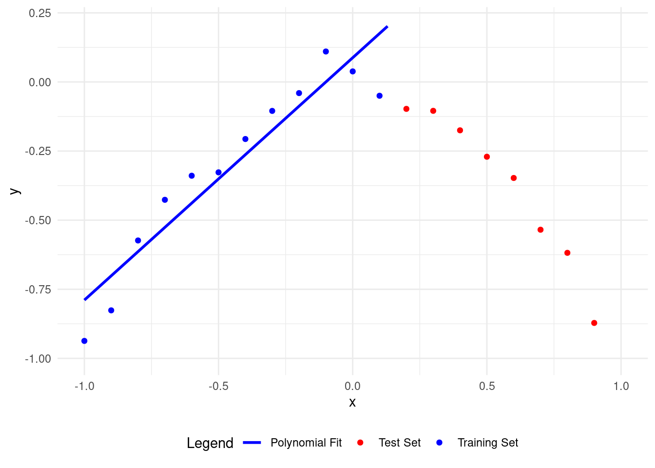
A polynomial of degree 1 fits the training data better than the test data, but it needs improvement. The model isn’t learning well from the training data, so it’s not good.
- Underfitting happens when a model is too simple to capture data patterns.
It performs poorly on both training and new data.
It fails to learn relationships, leading to inaccurate predictions.
- Underfitting can occur when:
The model is too simple (e.g., using a linear model for non-linear data).
There is not enough training data.
The model is not trained long enough.
- To avoid underfitting:
- Choose a model complex enough to capture data patterns but not too complex to overfit.
- 過度簡化發生在模型過於簡單,無法捕捉數據模式時。
它在訓練數據和新數據上表現不佳。
它無法學習關係,導致預測不準確。
- 過度簡化可能發生在:
模型過於簡單(例如,對非線性數據使用線性模型)。
訓練數據不足。
模型訓練時間不夠長。
- 為了避免過度簡化:
- 選擇一個足夠複雜以捕捉數據模式但不會過度擬合的模型。
Now, let’s see what happens with a high-degree polynomial.
Here’s a polynomial of degree \(7\).
# Load necessary libraries
library(ggplot2)

# Set seed for reproducibility
set.seed(0)

# Generate data
x <- seq(-1, 1, by = 0.1)
y <- -x^2 + rnorm(length(x), mean = 0, sd = 0.05)

# Create a data frame
data <- data.frame(x = x, y = y)

# Split data into training and test sets
train_data <- data[1:12, ]
test_data <- data[13:nrow(data), ]

# Polynomial fit function
polynomial_fit <- function(degree = 7) {
  lm(y ~ poly(x, degree), data = train_data)
}

# Plot polynomial fit
plot_polyfit <- function(degree = 7) {
  fit <- polynomial_fit(degree)
  curve_x <- seq(min(x), max(x), by = 0.01)
  curve_y <- predict(fit, newdata = data.frame(x = curve_x))

  ggplot() +
    geom_point(data = train_data, aes(x = x, y = y, color = "Training Set")) +
    geom_point(data = test_data, aes(x = x, y = y, color = "Test Set")) +
    geom_line(aes(x = curve_x, y = curve_y, color = "Polynomial Fit"), size = 1) +
    xlim(-1, 1) +
    ylim(-1, max(y) + 0.1) +
    labs(x = "x", y = "y") +
    theme_minimal() +
    theme(legend.position = "bottom") +
    scale_color_manual(name = "Legend",
                       values = c("Training Set" = "blue",
                                  "Test Set" = "red",
                                  "Polynomial Fit" = "blue"))
}

# Plot polynomial fit of degree 7
plot_polyfit(7)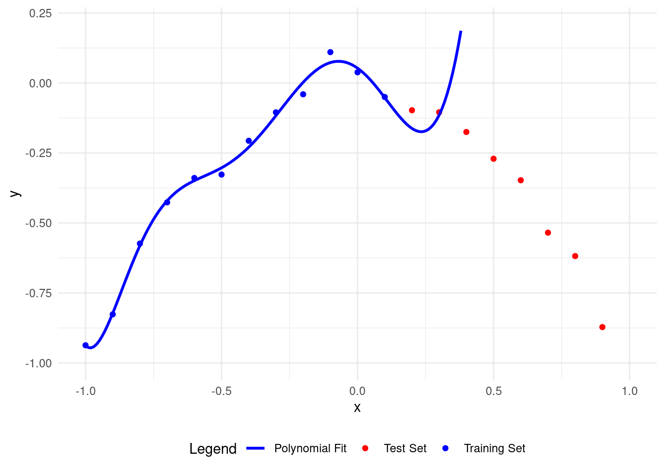
Here’s what happens with a polynomial of degree 11.
# Load necessary libraries
library(ggplot2)

# Set seed for reproducibility
set.seed(0)

# Generate data
x <- seq(-1, 1, by = 0.1)
y <- -x^2 + rnorm(length(x), mean = 0, sd = 0.05)

# Create a data frame
data <- data.frame(x = x, y = y)

# Split data into training and test sets
train_data <- data[1:12, ]
test_data <- data[13:nrow(data), ]

# Polynomial fit function
polynomial_fit <- function(degree = 11) {
  lm(y ~ poly(x, degree), data = train_data)
}

# Plot polynomial fit
plot_polyfit <- function(degree = 11) {
  fit <- polynomial_fit(degree)
  curve_x <- seq(min(x), max(x), by = 0.01)
  curve_y <- predict(fit, newdata = data.frame(x = curve_x))

  ggplot() +
    geom_point(data = train_data, aes(x = x, y = y, color = "Training Set")) +
    geom_point(data = test_data, aes(x = x, y = y, color = "Test Set")) +
    geom_line(aes(x = curve_x, y = curve_y, color = "Polynomial Fit"), size = 1) +
    xlim(-1, 1) +
    ylim(-1, max(y) + 0.1) +
    labs(x = "x", y = "y") +
    theme_minimal() +
    theme(legend.position = "bottom") +
    scale_color_manual(name = "Legend",
                       values = c("Training Set" = "blue",
                                  "Test Set" = "red",
                                  "Polynomial Fit" = "blue"))
}

# Plot polynomial fit of degree 11
plot_polyfit(11)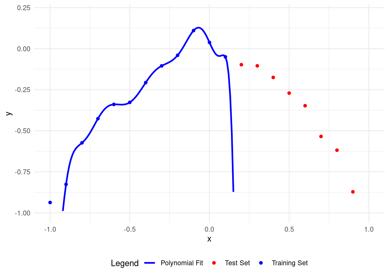
Now the polynomial fits the training points well but is wrong for the test points.
A higher degree polynomial causes overfitting and low accuracy on test data. More parameters make it more complex.
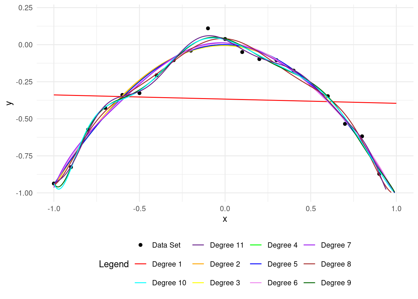
Let’s see overfitting clearly. With \(12\) training points, we can easily overfit using a polynomial of degree 11, called the Lagrange polynomial.
The polynomial fits the training data perfectly but is inaccurate on the test set.
A higher polynomial degree fits the training data better but performs worse on the test data.
多項式完美地擬合了訓練數據,但在測試集上不準確。
更高次數的多項式在訓練數據上擬合得更好,但在測試數據上表現更差。
The keyword is interpolation. We don’t want to interpolate because it fits errors as if they were useful data. We want to understand the model within the errors. A perfect fit results in a poor model for unseen data that follows the same patterns as the training data.
6 How to avoid overfitting
How do we find the right polynomial degree? Cross-validation helps. We measure the Root Mean Squared Error (RMSE) on the test data and choose the degree that minimizes this error.
我們如何找到合適的多項式次數?交叉驗證有幫助。
我們測量測試數據的均方根誤差\(\textrm{MSE}\),並選擇使此誤差最小的次數。
The Mean Square Error is defined as: \[ \textrm{MSE} = \dfrac{1}{N} \sum_{i=1}^{N} \left(\widehat{Y}_i - Y_i \right)^2 \] where
\(N\) is the size of the sample,
\(\widehat{Y}_i\) is the ith prediction (scalar real value), and
\(Y_i\) is the cor responding observation.
\(\sqrt{MSE}\) penalizes larger errors (sensitive to outliers).
Here are other error metrics:
這裡有其他的誤差度量指標
The Root Mean Square Error is defined as: \[ \textrm{RMSE} = \sqrt{MSE} \] where
- It has the same units as \(Y\).
The Normalized-Mean-Square Error is defined as: \[ \textrm{MAE} = \dfrac{\textrm{RMSE}}{\overline{Y}} \]
where
- \(\overline{Y}\) is either defined as the mean of \(Y\) or its range \({Y}_{\max} - {Y}_{\min}\).
The Mean Absolute Error is defined as
\[ \textrm{MAE} = \dfrac{1}{N} \sum_{i=1}^{N} \left| \widehat{Y}_i - Y_i \right| \]
MAE penalizes all errors equally: it is less sensitive to outliers than MSE.
The Average Relative Error is defined as:
\[ \textrm{ARE} = \dfrac{1}{N} \sum_{i=1}^{N} \dfrac{\left| \widehat{Y}_i - Y_i \right|}{|Y_i|} \]
# Load necessary libraries
library(ggplot2)
library(dplyr)

# Set seed for reproducibility
set.seed(0)

# Generate data
x <- seq(-1, 1, by = 0.1)
y <- -x^2 + rnorm(length(x), mean = 0, sd = 0.05)

# Create a data frame
data <- data.frame(x = x, y = y)

# Split data into training and test sets
X_train <- data[1:12, ]
X_test <- data[13:nrow(data), ]

# Polynomial fit function
polynomial_fit <- function(degree = 1) {
  lm(y ~ poly(x, degree), data = X_train)
}

# Function to calculate RMSE
calculate_rmse <- function(model, data) {
  predictions <- predict(model, newdata = data)
  sqrt(mean((data$y - predictions)^2))
}

# Store results
results <- data.frame(degree = integer(),
                      rmse_training = numeric(),
                      rmse_test = numeric())

# Loop through polynomial degrees
for (i in 1:(nrow(X_train) - 1)) {
  fit <- polynomial_fit(i)
  rmse_training <- calculate_rmse(fit, X_train)
  rmse_test <- calculate_rmse(fit, X_test)
  results <- rbind(results, data.frame(degree = i,
                                        rmse_training = rmse_training,
                                        rmse_test = rmse_test))
}

# Plotting the polynomial fit and RMSE
plot_polyfit <- function(degree = 1) {
  fit <- polynomial_fit(degree)
  curve_x <- seq(min(x), max(x), by = 0.01)
  curve_y <- predict(fit, newdata = data.frame(x = curve_x))

  ggplot() +
    geom_point(data = X_train, aes(x = x, y = y, color = "Training Set")) +
    geom_point(data = X_test, aes(x = x, y = y, color = "Test Set")) +
    geom_line(aes(x = curve_x, y = curve_y, color = "Polynomial Fit"), size = 1) +
    xlim(-1, 1) +
    ylim(-1, max(y) + 0.1) +
    labs(x = "x", y = "y") +
    theme_minimal() +
    theme(legend.position = "bottom") +
    scale_color_manual(name = "Legend",
                       values = c("Training Set" = "blue",
                                  "Test Set" = "red",
                                  "Polynomial Fit" = "green"))

  print(ggplot() +
          geom_point(data = results, aes(x = degree, y = rmse_training, color = "RMSE on Training")) +
          geom_point(data = results, aes(x = degree, y = rmse_test, color = "RMSE on Test")) +
          scale_y_log10() +
          labs(x = "Polynomial Degree", y = "RMSE") +
          theme_minimal() +
          theme(legend.position = "bottom") +
          scale_color_manual(name = "Legend",
                             values = c("RMSE on Training" = "blue",
                                        "RMSE on Test" = "red"))
  )
}

# Plot polynomial fit of degree 1
plot_polyfit(1)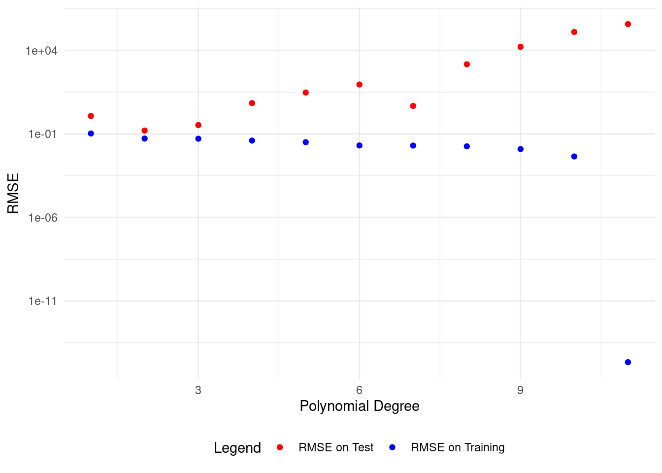
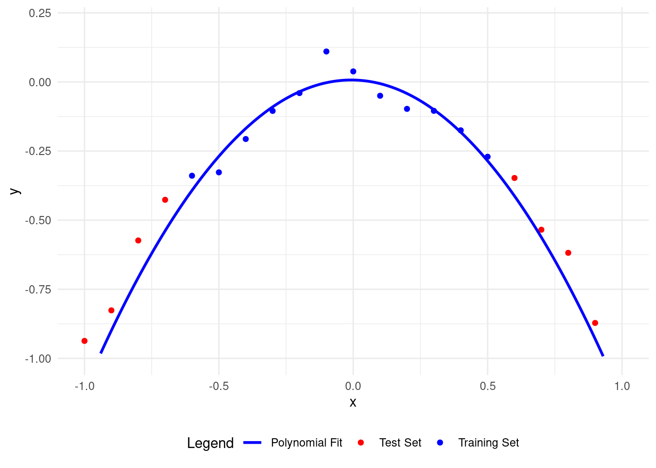
We get the lowest test set RMSE with a polynomial of degree 2, matching our data model.
This model describes both the training and test data well.
To generalize patterns in our data, we need to cross-validate our model on unseen data. This helps avoid overfitting.
我們使用二次多項式獲得了最低的測試集均方根誤差\(\textrm{MSE}\),與我們的數據模型相匹配。
這個模型很好地描述了訓練數據和測試數據。
為了在數據中概括模式,我們需要在未見過的數據上對模型進行交叉驗證。這有助於避免過度擬合。
# Load necessary libraries
library(ggplot2)

# Set seed for reproducibility
set.seed(0)

# Generate data
x <- seq(-1, 1, by = 0.1)
y <- -x^2 + rnorm(length(x), mean = 0, sd = 0.05)

# Create a data frame
data <- data.frame(x = x, y = y)

# Split data into training and test sets
train_data <- data[1:12, ]
test_data <- data[13:nrow(data), ]

# Polynomial fit function
polynomial_fit <- function(degree = 2) {
  lm(y ~ poly(x, degree), data = train_data)
}

# Plot polynomial fit
plot_polyfit <- function(degree = 2) {
  fit <- polynomial_fit(degree)
  curve_x <- seq(min(x), max(x), by = 0.01)
  curve_y <- predict(fit, newdata = data.frame(x = curve_x))

  ggplot() +
    geom_point(data = train_data, aes(x = x, y = y, color = "Training Set")) +
    geom_point(data = test_data, aes(x = x, y = y, color = "Test Set")) +
    geom_line(aes(x = curve_x, y = curve_y, color = "Polynomial Fit"), size = 1) +
    xlim(-1, 1) +
    ylim(-1, max(y) + 0.1) +
    labs(x = "x", y = "y") +
    theme_minimal() +
    theme(legend.position = "bottom") +
    scale_color_manual(name = "Legend",
                       values = c("Training Set" = "blue",
                                  "Test Set" = "red",
                                  "Polynomial Fit" = "blue"))
}

# Plot polynomial fit of degree 2
plot_polyfit(2)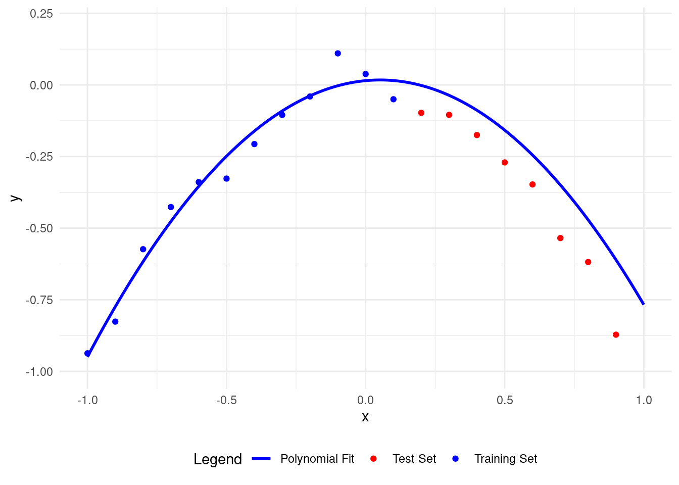
7 Performing the cross-validation calculations in Fold 2
Let’s split this dataset into training and test.
\[ \begin{array}{cc|c|c} \textrm{Fold 2}& \color{red}{\textrm{Test Data}} & \color{blue}{\textrm{Training Data}} & \color{red}{\textrm{Test Data}} \\ \hline & 1:4 & 5:16 & 17:21\\ \end{array} \]
Here’s what happens with a polynomial of degree 1.
# Load necessary libraries
library(ggplot2)

# Set seed for reproducibility
set.seed(0)

# Generate data
x <- seq(-1, 1, by = 0.1)
y <- -x^2 + rnorm(length(x), mean = 0, sd = 0.05)

# Create a data frame
data <- data.frame(x = x, y = y)

# Split data into training and test sets
train_data <- data[5:16, ]  # Points 5 to 16 as training set
test_data <- data[c(1:4, 17:21), ]  # Points 1 to 4 and 17 to 21 as test set

# Polynomial fit function
polynomial_fit <- function(degree = 1) {
  lm(y ~ poly(x, degree), data = train_data)
}

# Plot polynomial fit
plot_polyfit <- function(degree = 1) {
  fit <- polynomial_fit(degree)
  curve_x <- seq(min(x), max(x), by = 0.01)
  curve_y <- predict(fit, newdata = data.frame(x = curve_x))

  ggplot() +
    geom_point(data = train_data, aes(x = x, y = y, color = "Training Set")) +
    geom_point(data = test_data, aes(x = x, y = y, color = "Test Set")) +
    geom_line(aes(x = curve_x, y = curve_y, color = "Polynomial Fit"), size = 1) +
    xlim(-1, 1) +
    ylim(-1, max(y) + 0.1) +
    labs(x = "x", y = "y") +
    theme_minimal() +
    theme(legend.position = "bottom") +
    scale_color_manual(name = "Legend",
                       values = c("Training Set" = "blue",
                                  "Test Set" = "red",
                                  "Polynomial Fit" = "blue"))
}

# Plot polynomial fit of degree 1
plot_polyfit(1)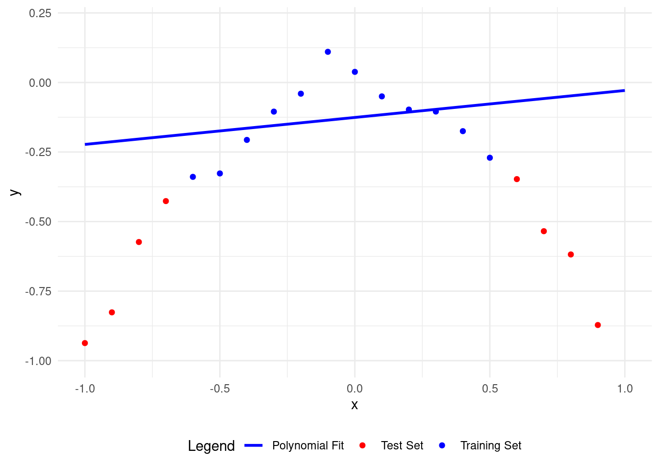
# Load necessary libraries
library(ggplot2)

# Set seed for reproducibility
set.seed(0)

# Generate data
x <- seq(-1, 1, by = 0.1)
y <- -x^2 + rnorm(length(x), mean = 0, sd = 0.05)

# Create a data frame
data <- data.frame(x = x, y = y)

# Split data into training and test sets
train_data <- data[5:16, ]  # Points 5 to 16 as training set
test_data <- data[c(1:4, 17:21), ]  # Points 1 to 4 and 17 to 21 as test set

# Polynomial fit function
polynomial_fit <- function(degree = 7) {
  lm(y ~ poly(x, degree), data = train_data)
}

# Plot polynomial fit
plot_polyfit <- function(degree = 7) {
  fit <- polynomial_fit(degree)
  curve_x <- seq(min(x), max(x), by = 0.01)
  curve_y <- predict(fit, newdata = data.frame(x = curve_x))

  ggplot() +
    geom_point(data = train_data, aes(x = x, y = y, color = "Training Set")) +
    geom_point(data = test_data, aes(x = x, y = y, color = "Test Set")) +
    geom_line(aes(x = curve_x, y = curve_y, color = "Polynomial Fit"), size = 1) +
    xlim(-1, 1) +
    ylim(-1, max(y) + 0.1) +
    labs(x = "x", y = "y") +
    theme_minimal() +
    theme(legend.position = "bottom") +
    scale_color_manual(name = "Legend",
                       values = c("Training Set" = "blue",
                                  "Test Set" = "red",
                                  "Polynomial Fit" = "blue"))
}

# Plot polynomial fit of degree 7
plot_polyfit(7)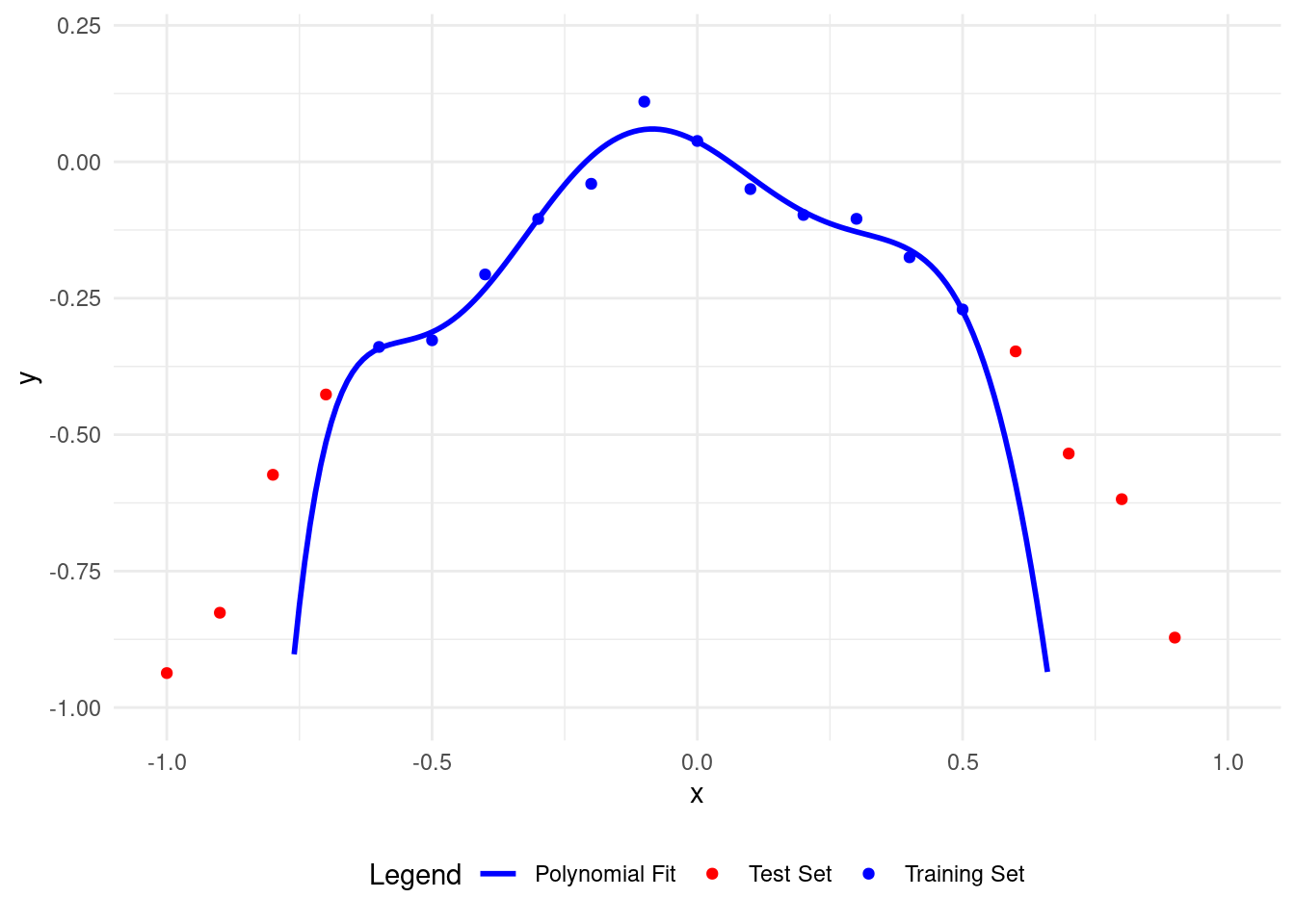
# Load necessary libraries
library(ggplot2)

# Set seed for reproducibility
set.seed(0)

# Generate data
x <- seq(-1, 1, by = 0.1)
y <- -x^2 + rnorm(length(x), mean = 0, sd = 0.05)

# Create a data frame
data <- data.frame(x = x, y = y)

# Split data into training and test sets
train_data <- data[5:16, ]  # Points 5 to 16 as training set
test_data <- data[c(1:4, 17:21), ]  # Points 1 to 4 and 17 to 21 as test set

# Polynomial fit function
polynomial_fit <- function(degree = 11) {
  lm(y ~ poly(x, degree), data = train_data)
}

# Plot polynomial fit
plot_polyfit <- function(degree = 11) {
  fit <- polynomial_fit(degree)
  curve_x <- seq(min(x), max(x), by = 0.01)
  curve_y <- predict(fit, newdata = data.frame(x = curve_x))

  ggplot() +
    geom_point(data = train_data, aes(x = x, y = y, color = "Training Set")) +
    geom_point(data = test_data, aes(x = x, y = y, color = "Test Set")) +
    geom_line(aes(x = curve_x, y = curve_y, color = "Polynomial Fit"), size = 1) +
    xlim(-1, 1) +
    ylim(-1, max(y) + 0.1) +
    labs(x = "x", y = "y") +
    theme_minimal() +
    theme(legend.position = "bottom") +
    scale_color_manual(name = "Legend",
                       values = c("Training Set" = "blue",
                                  "Test Set" = "red",
                                  "Polynomial Fit" = "blue"))
}

# Plot polynomial fit of degree 11
plot_polyfit(11)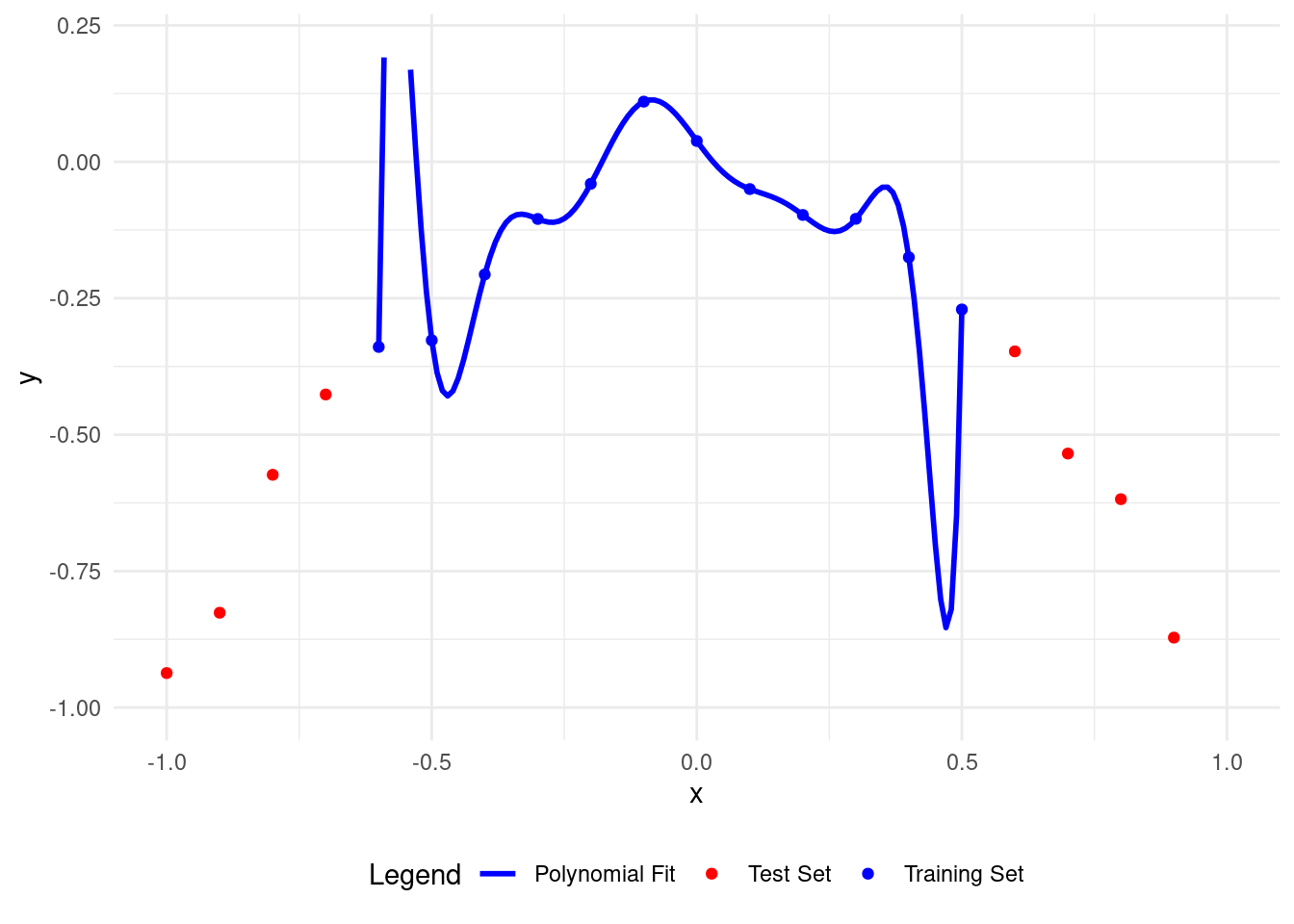
# Load necessary libraries
library(ggplot2)
library(dplyr)

# Set seed for reproducibility
set.seed(0)

# Generate data
x <- seq(-1, 1, by = 0.1)
y <- -x^2 + rnorm(length(x), mean = 0, sd = 0.05)

# Create a data frame
data <- data.frame(x = x, y = y)

# Split data into training and test sets
X_train <- data[5:16, ]  # Points 5 to 16 as training set
X_test <- data[c(1:4, 17:21), ]  # Points 1 to 4 and 17 to 21 as test set


# Polynomial fit function
polynomial_fit <- function(degree = 1) {
  lm(y ~ poly(x, degree), data = X_train)
}

# Function to calculate RMSE
calculate_rmse <- function(model, data) {
  predictions <- predict(model, newdata = data)
  sqrt(mean((data$y - predictions)^2))
}

# Store results
results <- data.frame(degree = integer(),
                      rmse_training = numeric(),
                      rmse_test = numeric())

# Loop through polynomial degrees
for (i in 1:(nrow(X_train) - 1)) {
  fit <- polynomial_fit(i)
  rmse_training <- calculate_rmse(fit, X_train)
  rmse_test <- calculate_rmse(fit, X_test)
  results <- rbind(results, data.frame(degree = i,
                                        rmse_training = rmse_training,
                                        rmse_test = rmse_test))
}

# Plotting the polynomial fit and RMSE
plot_polyfit <- function(degree = 1) {
  fit <- polynomial_fit(degree)
  curve_x <- seq(min(x), max(x), by = 0.01)
  curve_y <- predict(fit, newdata = data.frame(x = curve_x))

  ggplot() +
    geom_point(data = X_train, aes(x = x, y = y, color = "Training Set")) +
    geom_point(data = X_test, aes(x = x, y = y, color = "Test Set")) +
    geom_line(aes(x = curve_x, y = curve_y, color = "Polynomial Fit"), size = 1) +
    xlim(-1, 1) +
    ylim(-1, max(y) + 0.1) +
    labs(x = "x", y = "y") +
    theme_minimal() +
    theme(legend.position = "bottom") +
    scale_color_manual(name = "Legend",
                       values = c("Training Set" = "blue",
                                  "Test Set" = "red",
                                  "Polynomial Fit" = "green"))

  print(ggplot() +
          geom_point(data = results, aes(x = degree, y = rmse_training, color = "RMSE on Training")) +
          geom_point(data = results, aes(x = degree, y = rmse_test, color = "RMSE on Test")) +
          scale_y_log10() +
          labs(x = "Polynomial Degree", y = "RMSE") +
          theme_minimal() +
          theme(legend.position = "bottom") +
          scale_color_manual(name = "Legend",
                             values = c("RMSE on Training" = "blue",
                                        "RMSE on Test" = "red"))
  )
}

# Plot polynomial fit of degree 1
plot_polyfit(1)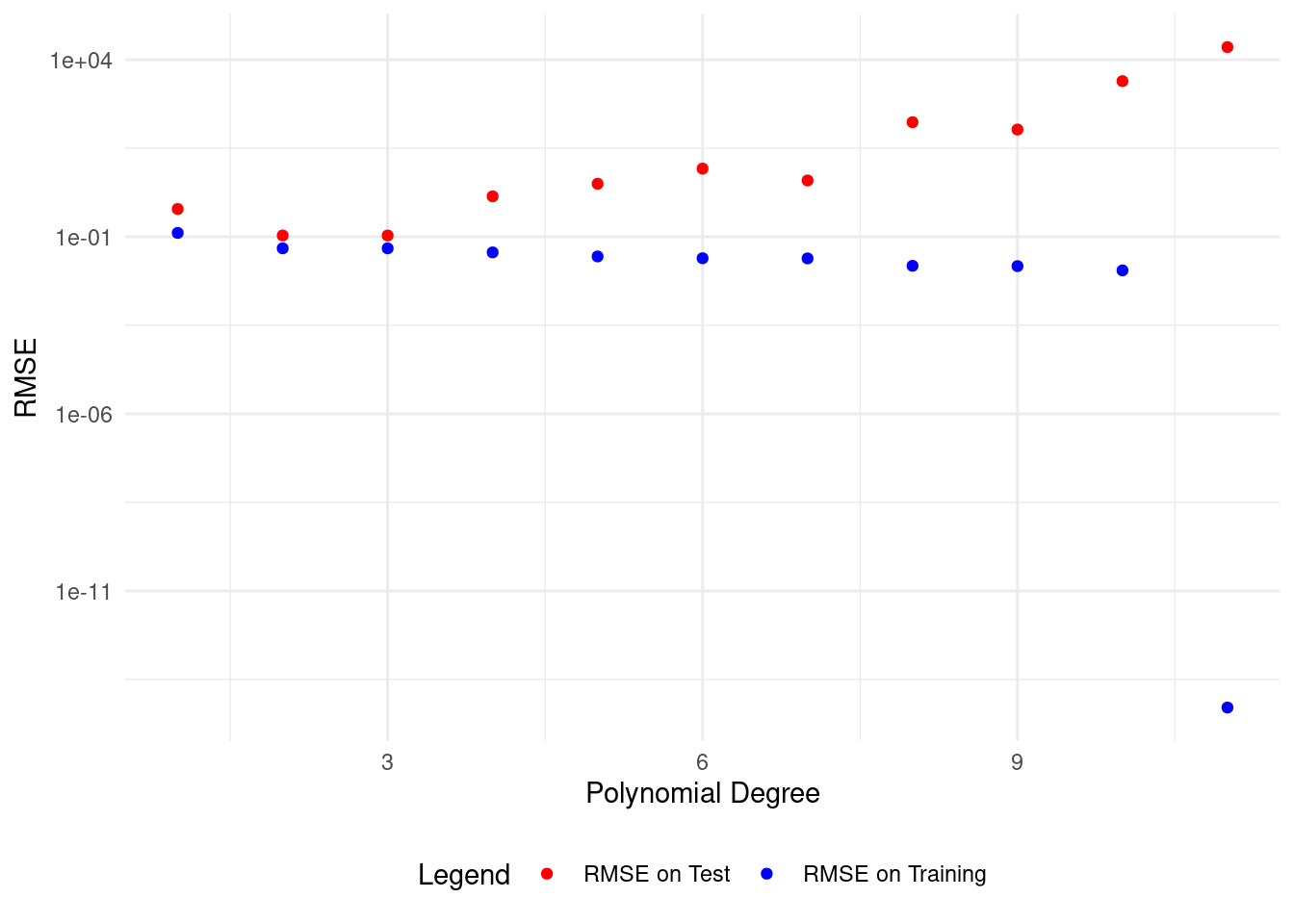
8 Performing the cross-validation calculations in Fold 3
Let’s split this dataset into training and test.
\[ \begin{array}{cc|c} \textrm{Fold 3} &\color{red}{\textrm{Test Data}} & \color{blue}{\textrm{Training Data}} \\ \hline & 1:9 & 10:21\\ \end{array} \]
Here’s what happens with a polynomial of degree 1.
# Load necessary libraries
library(ggplot2)

# Set seed for reproducibility
set.seed(0)

# Generate data
x <- seq(-1, 1, by = 0.1)
y <- -x^2 + rnorm(length(x), mean = 0, sd = 0.05)

# Create a data frame
data <- data.frame(x = x, y = y)

# Split data into training and test sets
train_data <- data[10:21, ]  # Points 9 to 21 as training set
test_data <- data[1:9, ]  # Points 1 to 9 as test set

# Polynomial fit function
polynomial_fit <- function(degree = 1) {
  lm(y ~ poly(x, degree), data = train_data)
}

# Plot polynomial fit
plot_polyfit <- function(degree = 1) {
  fit <- polynomial_fit(degree)
  curve_x <- seq(min(x), max(x), by = 0.01)
  curve_y <- predict(fit, newdata = data.frame(x = curve_x))

  ggplot() +
    geom_point(data = train_data, aes(x = x, y = y, color = "Training Set")) +
    geom_point(data = test_data, aes(x = x, y = y, color = "Test Set")) +
    geom_line(aes(x = curve_x, y = curve_y, color = "Polynomial Fit"), size = 1) +
    xlim(-1, 1) +
    ylim(-1, max(y) + 0.1) +
    labs(x = "x", y = "y") +
    theme_minimal() +
    theme(legend.position = "bottom") +
    scale_color_manual(name = "Legend",
                       values = c("Training Set" = "blue",
                                  "Test Set" = "red",
                                  "Polynomial Fit" = "blue"))
}

# Plot polynomial fit of degree 1
plot_polyfit(1)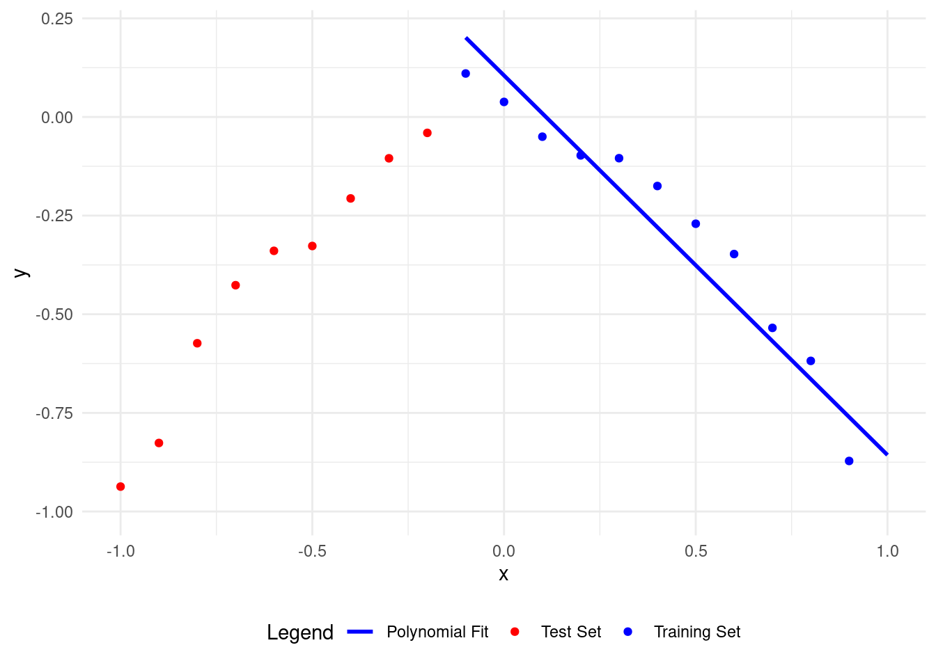
# Load necessary libraries
library(ggplot2)

# Set seed for reproducibility
set.seed(0)

# Generate data
x <- seq(-1, 1, by = 0.1)
y <- -x^2 + rnorm(length(x), mean = 0, sd = 0.05)

# Create a data frame
data <- data.frame(x = x, y = y)

# Split data into training and test sets
train_data <- data[10:21, ]  # Points 9 to 21 as training set
test_data <- data[1:9, ]  # Points 1 to 9 as test set


# Polynomial fit function
polynomial_fit <- function(degree = 7) {
  lm(y ~ poly(x, degree), data = train_data)
}

# Plot polynomial fit
plot_polyfit <- function(degree = 7) {
  fit <- polynomial_fit(degree)
  curve_x <- seq(min(x), max(x), by = 0.01)
  curve_y <- predict(fit, newdata = data.frame(x = curve_x))

  ggplot() +
    geom_point(data = train_data, aes(x = x, y = y, color = "Training Set")) +
    geom_point(data = test_data, aes(x = x, y = y, color = "Test Set")) +
    geom_line(aes(x = curve_x, y = curve_y, color = "Polynomial Fit"), size = 1) +
    xlim(-1, 1) +
    ylim(-1, max(y) + 0.1) +
    labs(x = "x", y = "y") +
    theme_minimal() +
    theme(legend.position = "bottom") +
    scale_color_manual(name = "Legend",
                       values = c("Training Set" = "blue",
                                  "Test Set" = "red",
                                  "Polynomial Fit" = "blue"))
}

# Plot polynomial fit of degree 7
plot_polyfit(7)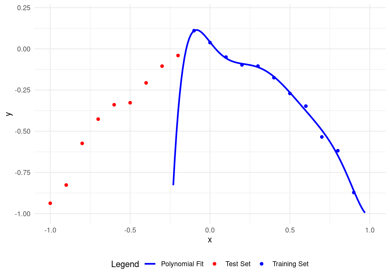
# Load necessary libraries
library(ggplot2)

# Set seed for reproducibility
set.seed(0)

# Generate data
x <- seq(-1, 1, by = 0.1)
y <- -x^2 + rnorm(length(x), mean = 0, sd = 0.05)

# Create a data frame
data <- data.frame(x = x, y = y)


# Split data into training and test sets
train_data <- data[10:21, ]  # Points 9 to 21 as training set
test_data <- data[1:9, ]  # Points 1 to 9 as test set


# Polynomial fit function
polynomial_fit <- function(degree = 11) {
  lm(y ~ poly(x, degree), data = train_data)
}

# Plot polynomial fit
plot_polyfit <- function(degree = 11) {
  fit <- polynomial_fit(degree)
  curve_x <- seq(min(x), max(x), by = 0.01)
  curve_y <- predict(fit, newdata = data.frame(x = curve_x))

  ggplot() +
    geom_point(data = train_data, aes(x = x, y = y, color = "Training Set")) +
    geom_point(data = test_data, aes(x = x, y = y, color = "Test Set")) +
    geom_line(aes(x = curve_x, y = curve_y, color = "Polynomial Fit"), size = 1) +
    xlim(-1, 1) +
    ylim(-1, max(y) + 0.1) +
    labs(x = "x", y = "y") +
    theme_minimal() +
    theme(legend.position = "bottom") +
    scale_color_manual(name = "Legend",
                       values = c("Training Set" = "blue",
                                  "Test Set" = "red",
                                  "Polynomial Fit" = "blue"))
}

# Plot polynomial fit of degree 11
plot_polyfit(11)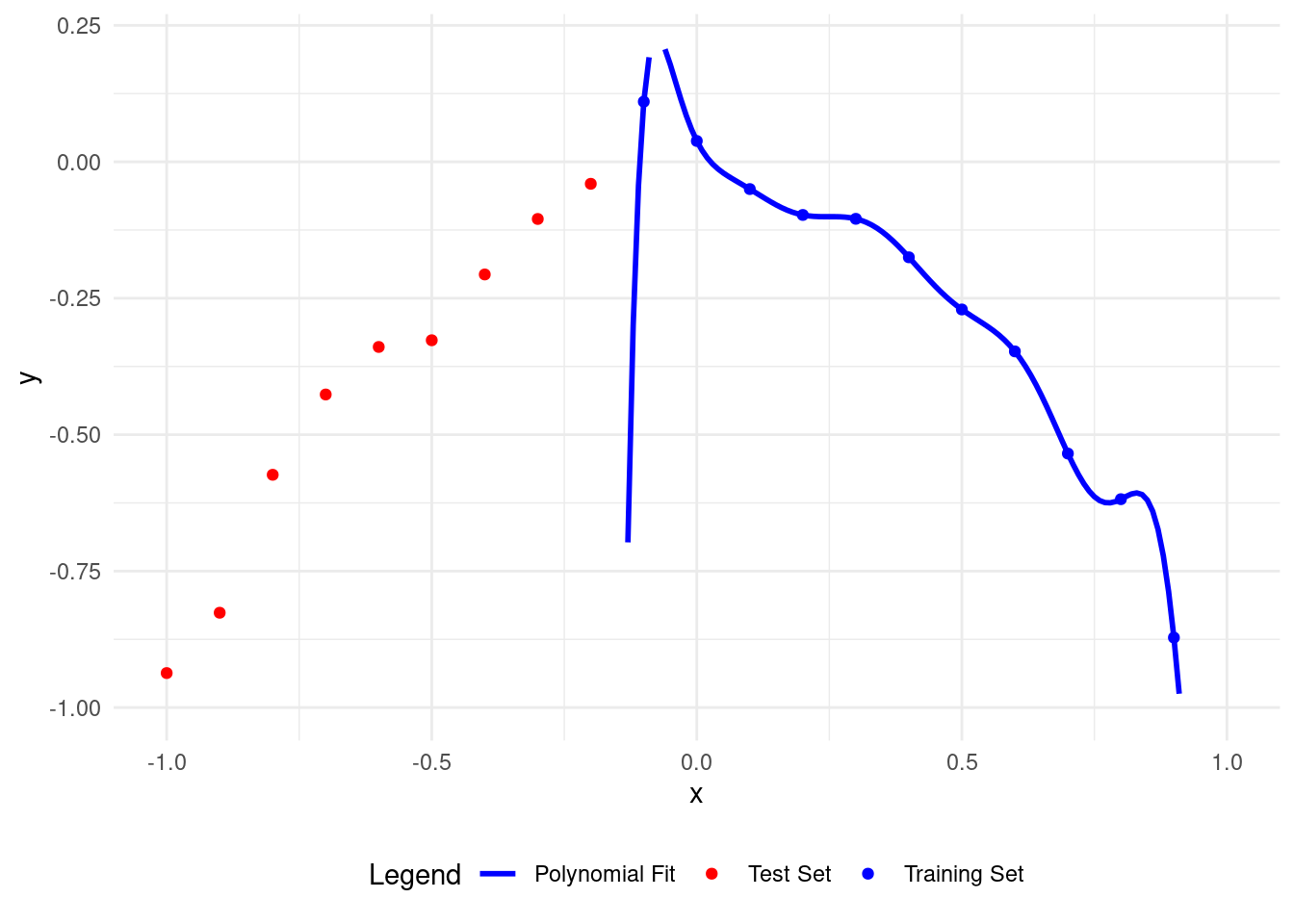
# Load necessary libraries
library(ggplot2)
library(dplyr)

# Set seed for reproducibility
set.seed(0)

# Generate data
x <- seq(-1, 1, by = 0.1)
y <- -x^2 + rnorm(length(x), mean = 0, sd = 0.05)

# Create a data frame
data <- data.frame(x = x, y = y)

# Split data into training and test sets
X_train <- data[9:21, ]  # Points 10 to 21 as training set
X_test <- data[1:8, ]  # Points 1 to 9 as test set


# Polynomial fit function
polynomial_fit <- function(degree = 1) {
  lm(y ~ poly(x, degree), data = X_train)
}

# Function to calculate RMSE
calculate_rmse <- function(model, data) {
  predictions <- predict(model, newdata = data)
  sqrt(mean((data$y - predictions)^2))
}

# Store results
results <- data.frame(degree = integer(),
                      rmse_training = numeric(),
                      rmse_test = numeric())

# Loop through polynomial degrees
for (i in 1:(nrow(X_train) - 1)) {
  fit <- polynomial_fit(i)
  rmse_training <- calculate_rmse(fit, X_train)
  rmse_test <- calculate_rmse(fit, X_test)
  results <- rbind(results, data.frame(degree = i,
                                        rmse_training = rmse_training,
                                        rmse_test = rmse_test))
}

# Plotting the polynomial fit and RMSE
plot_polyfit <- function(degree = 1) {
  fit <- polynomial_fit(degree)
  curve_x <- seq(min(x), max(x), by = 0.01)
  curve_y <- predict(fit, newdata = data.frame(x = curve_x))

  ggplot() +
    geom_point(data = X_train, aes(x = x, y = y, color = "Training Set")) +
    geom_point(data = X_test, aes(x = x, y = y, color = "Test Set")) +
    geom_line(aes(x = curve_x, y = curve_y, color = "Polynomial Fit"), size = 1) +
    xlim(-1, 1) +
    ylim(-1, max(y) + 0.1) +
    labs(x = "x", y = "y") +
    theme_minimal() +
    theme(legend.position = "bottom") +
    scale_color_manual(name = "Legend",
                       values = c("Training Set" = "blue",
                                  "Test Set" = "red",
                                  "Polynomial Fit" = "green"))

  print(ggplot() +
          geom_point(data = results, aes(x = degree, y = rmse_training, color = "RMSE on Training")) +
          geom_point(data = results, aes(x = degree, y = rmse_test, color = "RMSE on Test")) +
          scale_y_log10() +
          labs(x = "Polynomial Degree", y = "RMSE") +
          theme_minimal() +
          theme(legend.position = "bottom") +
          scale_color_manual(name = "Legend",
                             values = c("RMSE on Training" = "blue",
                                        "RMSE on Test" = "red"))
  )
}

# Plot polynomial fit of degree 1
plot_polyfit(1)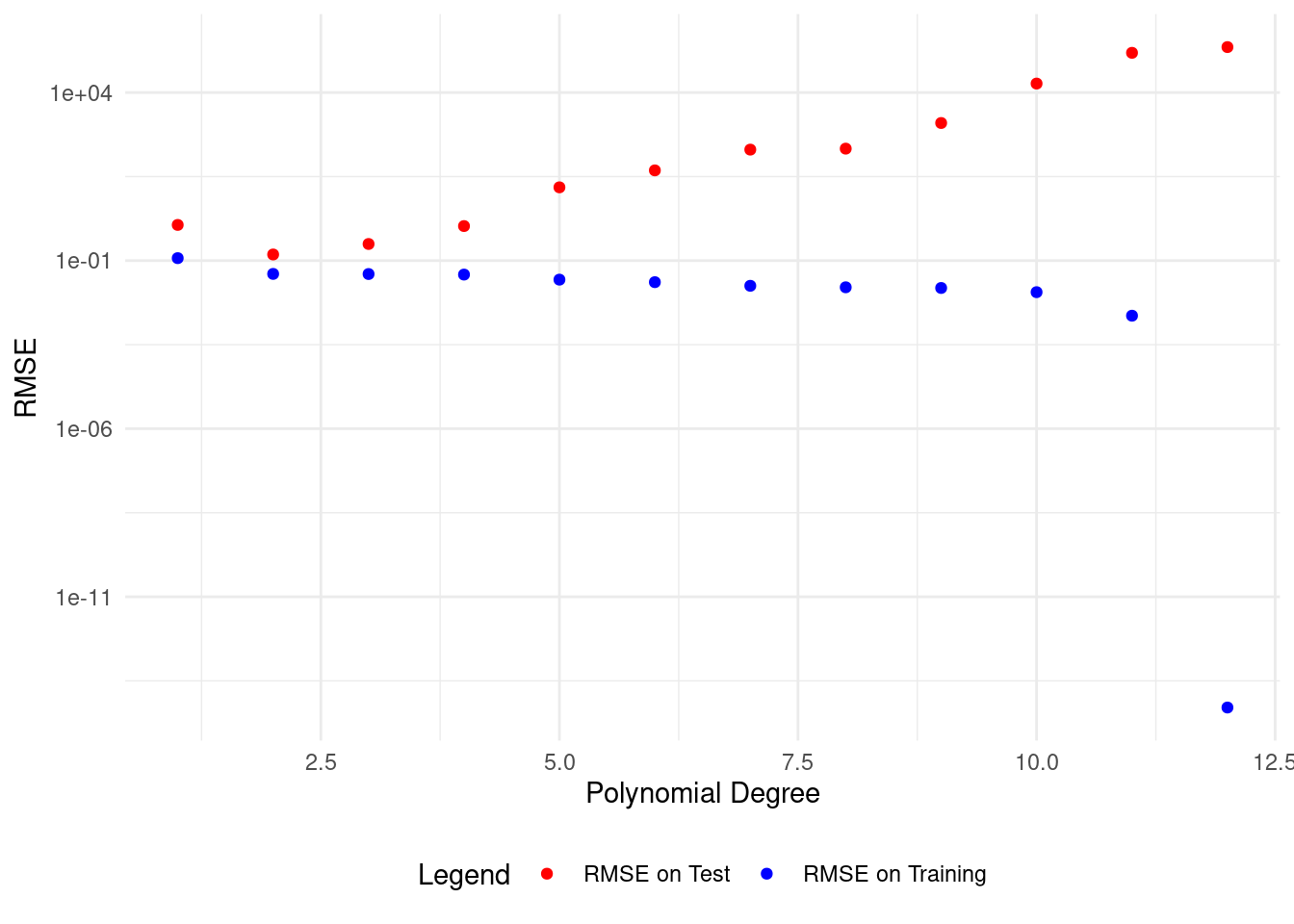

9 More sample points with 5 folds
Let us create 100 points following the equation: \[ Y = - X^2 \]
Each point will have a normally distributed error with a mean of \(0\) and a standard deviation of \(0.05\). In real-life data science, data always has some random error.
We’ll use the first \(20\) points as the training set and the last \(80\) points as the test set.
Five folds are considered.
A comparison of four error metrics is used.
考慮了五個折疊。
使用了四個誤差度量指標的比較。
\[ \begin{array}{cc|c} \textrm{Fold 1}&\color{blue}{\textrm{Training Data}} & \color{red}{\textrm{Test Data}} \\ \hline &1:20 & 21:100\\ \end{array} \] \[ \begin{array}{cc|c|c} \textrm{Fold 2}& \color{red}{\textrm{Test Data}} & \color{blue}{\textrm{Training Data}} & \color{red}{\textrm{Test Data}} \\ \hline & 1:20 & 21:40 & 41:100\\ \end{array} \] \[ \begin{array}{cc|c|c} \textrm{Fold 3}& \color{red}{\textrm{Test Data}} & \color{blue}{\textrm{Training Data}} & \color{red}{\textrm{Test Data}} \\ \hline & 1:40 & 41:60 & 61:100\\ \end{array} \] \[ \begin{array}{cc|c|c} \textrm{Fold 4}& \color{red}{\textrm{Test Data}} & \color{blue}{\textrm{Training Data}} & \color{red}{\textrm{Test Data}} \\ \hline & 1:60 & 61:80 & 81:100\\ \end{array} \] \[ \begin{array}{cc|c} \textrm{Fold 5}&\color{blue}{\textrm{Training Data}} & \color{red}{\textrm{Test Data}} \\ \hline &1:80 & 81:100\\ \end{array} \]
Fold 1:
| degree | rmse_training | rmse_test | nrmse_training | nrmse_test | mae_training | mae_test | are_training | are_test |
|---|---|---|---|---|---|---|---|---|
| 1 | 0.0471529 | 1.388947e+00 | 0.0471529 | 1.388947e+00 | 0.0471529 | 1.388947e+00 | 0.0471529 | 1.388947e+00 |
| 2 | 0.0463135 | 2.535848e-01 | 0.0463135 | 2.535848e-01 | 0.0463135 | 2.535848e-01 | 0.0463135 | 2.535848e-01 |
| 3 | 0.0457318 | 1.399802e+01 | 0.0457318 | 1.399802e+01 | 0.0457318 | 1.399802e+01 | 0.0457318 | 1.399802e+01 |
| 4 | 0.0456674 | 6.183825e+01 | 0.0456674 | 6.183825e+01 | 0.0456674 | 6.183825e+01 | 0.0456674 | 6.183825e+01 |
| 5 | 0.0456033 | 1.196970e+03 | 0.0456033 | 1.196970e+03 | 0.0456033 | 1.196970e+03 | 0.0456033 | 1.196970e+03 |
| 6 | 0.0419949 | 1.607139e+05 | 0.0419949 | 1.607139e+05 | 0.0419949 | 1.607139e+05 | 0.0419949 | 1.607139e+05 |
| 7 | 0.0417363 | 9.031638e+05 | 0.0417363 | 9.031638e+05 | 0.0417363 | 9.031638e+05 | 0.0417363 | 9.031638e+05 |
| 8 | 0.0347502 | 6.684316e+07 | 0.0347502 | 6.684316e+07 | 0.0347502 | 6.684316e+07 | 0.0347502 | 6.684316e+07 |
| 9 | 0.0239069 | 1.336346e+09 | 0.0239069 | 1.336346e+09 | 0.0239069 | 1.336346e+09 | 0.0239069 | 1.336346e+09 |
| 10 | 0.0213521 | 1.311644e+10 | 0.0213521 | 1.311644e+10 | 0.0213521 | 1.311644e+10 | 0.0213521 | 1.311644e+10 |
| 11 | 0.0212449 | 3.496080e+10 | 0.0212449 | 3.496080e+10 | 0.0212449 | 3.496080e+10 | 0.0212449 | 3.496080e+10 |
| 12 | 0.0211573 | 9.670621e+11 | 0.0211573 | 9.670621e+11 | 0.0211573 | 9.670621e+11 | 0.0211573 | 9.670621e+11 |
| 13 | 0.0198628 | 7.912955e+13 | 0.0198628 | 7.912955e+13 | 0.0198628 | 7.912955e+13 | 0.0198628 | 7.912955e+13 |
| 14 | 0.0158664 | 3.264973e+15 | 0.0158664 | 3.264973e+15 | 0.0158664 | 3.264973e+15 | 0.0158664 | 3.264973e+15 |
| 15 | 0.0150261 | 3.893437e+16 | 0.0150261 | 3.893437e+16 | 0.0150261 | 3.893437e+16 | 0.0150261 | 3.893437e+16 |
| 16 | 0.0102441 | 2.194155e+18 | 0.0102441 | 2.194155e+18 | 0.0102441 | 2.194155e+18 | 0.0102441 | 2.194155e+18 |
| 17 | 0.0086420 | 3.481412e+19 | 0.0086420 | 3.481412e+19 | 0.0086420 | 3.481412e+19 | 0.0086420 | 3.481412e+19 |
| 18 | 0.0080237 | 9.008780e+20 | 0.0080237 | 9.008780e+20 | 0.0080237 | 9.008780e+20 | 0.0080237 | 9.008780e+20 |
| 19 | 0.0000000 | 1.205001e+23 | 0.0000000 | 1.205001e+23 | 0.0000000 | 1.205001e+23 | 0.0000000 | 1.205001e+23 |
Fold 2:
| degree | rmse_training | rmse_test | nrmse_training | nrmse_test | mae_training | mae_test | are_training | are_test |
|---|---|---|---|---|---|---|---|---|
| 1 | 0.0337162 | 8.516042e-01 | 0.0337162 | 8.516042e-01 | 0.0337162 | 8.516042e-01 | 0.0337162 | 8.516042e-01 |
| 2 | 0.0335878 | 6.496613e-01 | 0.0335878 | 6.496613e-01 | 0.0335878 | 6.496613e-01 | 0.0335878 | 6.496613e-01 |
| 3 | 0.0335834 | 1.077356e+00 | 0.0335834 | 1.077356e+00 | 0.0335834 | 1.077356e+00 | 0.0335834 | 1.077356e+00 |
| 4 | 0.0278528 | 1.862101e+02 | 0.0278528 | 1.862101e+02 | 0.0278528 | 1.862101e+02 | 0.0278528 | 1.862101e+02 |
| 5 | 0.0276613 | 6.067066e+02 | 0.0276613 | 6.067066e+02 | 0.0276613 | 6.067066e+02 | 0.0276613 | 6.067066e+02 |
| 6 | 0.0274134 | 5.785460e+03 | 0.0274134 | 5.785460e+03 | 0.0274134 | 5.785460e+03 | 0.0274134 | 5.785460e+03 |
| 7 | 0.0274009 | 2.557697e+04 | 0.0274009 | 2.557697e+04 | 0.0274009 | 2.557697e+04 | 0.0274009 | 2.557697e+04 |
| 8 | 0.0271184 | 1.310073e+06 | 0.0271184 | 1.310073e+06 | 0.0271184 | 1.310073e+06 | 0.0271184 | 1.310073e+06 |
| 9 | 0.0269564 | 1.615317e+07 | 0.0269564 | 1.615317e+07 | 0.0269564 | 1.615317e+07 | 0.0269564 | 1.615317e+07 |
| 10 | 0.0229599 | 1.099367e+09 | 0.0229599 | 1.099367e+09 | 0.0229599 | 1.099367e+09 | 0.0229599 | 1.099367e+09 |
| 11 | 0.0173943 | 1.941368e+10 | 0.0173943 | 1.941368e+10 | 0.0173943 | 1.941368e+10 | 0.0173943 | 1.941368e+10 |
| 12 | 0.0173776 | 3.497622e+10 | 0.0173776 | 3.497622e+10 | 0.0173776 | 3.497622e+10 | 0.0173776 | 3.497622e+10 |
| 13 | 0.0161767 | 2.252477e+12 | 0.0161767 | 2.252477e+12 | 0.0161767 | 2.252477e+12 | 0.0161767 | 2.252477e+12 |
| 14 | 0.0105406 | 8.106127e+13 | 0.0105406 | 8.106127e+13 | 0.0105406 | 8.106127e+13 | 0.0105406 | 8.106127e+13 |
| 15 | 0.0095789 | 5.281931e+14 | 0.0095789 | 5.281931e+14 | 0.0095789 | 5.281931e+14 | 0.0095789 | 5.281931e+14 |
| 16 | 0.0093641 | 6.826138e+15 | 0.0093641 | 6.826138e+15 | 0.0093641 | 6.826138e+15 | 0.0093641 | 6.826138e+15 |
| 17 | 0.0029668 | 7.068569e+17 | 0.0029668 | 7.068569e+17 | 0.0029668 | 7.068569e+17 | 0.0029668 | 7.068569e+17 |
| 18 | 0.0014204 | 7.229785e+18 | 0.0014204 | 7.229785e+18 | 0.0014204 | 7.229785e+18 | 0.0014204 | 7.229785e+18 |
| 19 | 0.0000000 | 1.478421e+20 | 0.0000000 | 1.478421e+20 | 0.0000000 | 1.478421e+20 | 0.0000000 | 1.478421e+20 |
Fold 3:
| degree | rmse_training | rmse_test | nrmse_training | nrmse_test | mae_training | mae_test | are_training | are_test |
|---|---|---|---|---|---|---|---|---|
| 1 | 0.0578638 | 4.930874e-01 | 0.0578638 | 4.930874e-01 | 0.0578638 | 4.930874e-01 | 0.0578638 | 4.930874e-01 |
| 2 | 0.0541416 | 3.617635e-01 | 0.0541416 | 3.617635e-01 | 0.0541416 | 3.617635e-01 | 0.0541416 | 3.617635e-01 |
| 3 | 0.0428585 | 1.142964e+01 | 0.0428585 | 1.142964e+01 | 0.0428585 | 1.142964e+01 | 0.0428585 | 1.142964e+01 |
| 4 | 0.0401145 | 4.688858e+01 | 0.0401145 | 4.688858e+01 | 0.0401145 | 4.688858e+01 | 0.0401145 | 4.688858e+01 |
| 5 | 0.0397461 | 1.689043e+02 | 0.0397461 | 1.689043e+02 | 0.0397461 | 1.689043e+02 | 0.0397461 | 1.689043e+02 |
| 6 | 0.0397377 | 2.380062e+02 | 0.0397377 | 2.380062e+02 | 0.0397377 | 2.380062e+02 | 0.0397377 | 2.380062e+02 |
| 7 | 0.0375354 | 3.387839e+04 | 0.0375354 | 3.387839e+04 | 0.0375354 | 3.387839e+04 | 0.0375354 | 3.387839e+04 |
| 8 | 0.0365379 | 2.296175e+05 | 0.0365379 | 2.296175e+05 | 0.0365379 | 2.296175e+05 | 0.0365379 | 2.296175e+05 |
| 9 | 0.0361500 | 1.522088e+06 | 0.0361500 | 1.522088e+06 | 0.0361500 | 1.522088e+06 | 0.0361500 | 1.522088e+06 |
| 10 | 0.0337690 | 3.914115e+07 | 0.0337690 | 3.914115e+07 | 0.0337690 | 3.914115e+07 | 0.0337690 | 3.914115e+07 |
| 11 | 0.0333405 | 1.888128e+08 | 0.0333405 | 1.888128e+08 | 0.0333405 | 1.888128e+08 | 0.0333405 | 1.888128e+08 |
| 12 | 0.0294302 | 6.326651e+09 | 0.0294302 | 6.326651e+09 | 0.0294302 | 6.326651e+09 | 0.0294302 | 6.326651e+09 |
| 13 | 0.0290610 | 2.436290e+10 | 0.0290610 | 2.436290e+10 | 0.0290610 | 2.436290e+10 | 0.0290610 | 2.436290e+10 |
| 14 | 0.0257248 | 9.193186e+11 | 0.0257248 | 9.193186e+11 | 0.0257248 | 9.193186e+11 | 0.0257248 | 9.193186e+11 |
| 15 | 0.0253478 | 4.436066e+12 | 0.0253478 | 4.436066e+12 | 0.0253478 | 4.436066e+12 | 0.0253478 | 4.436066e+12 |
| 16 | 0.0250259 | 6.353953e+13 | 0.0250259 | 6.353953e+13 | 0.0250259 | 6.353953e+13 | 0.0250259 | 6.353953e+13 |
| 17 | 0.0250198 | 1.697835e+14 | 0.0250198 | 1.697835e+14 | 0.0250198 | 1.697835e+14 | 0.0250198 | 1.697835e+14 |
| 18 | 0.0112042 | 1.456955e+17 | 0.0112042 | 1.456955e+17 | 0.0112042 | 1.456955e+17 | 0.0112042 | 1.456955e+17 |
| 19 | 0.0000000 | 2.272735e+18 | 0.0000000 | 2.272735e+18 | 0.0000000 | 2.272735e+18 | 0.0000000 | 2.272735e+18 |
Fold 4:
| degree | rmse_training | rmse_test | nrmse_training | nrmse_test | mae_training | mae_test | are_training | are_test |
|---|---|---|---|---|---|---|---|---|
| 1 | 0.0380707 | 8.312129e-01 | 0.0380707 | 8.312129e-01 | 0.0380707 | 8.312129e-01 | 0.0380707 | 8.312129e-01 |
| 2 | 0.0313535 | 6.584882e-01 | 0.0313535 | 6.584882e-01 | 0.0313535 | 6.584882e-01 | 0.0313535 | 6.584882e-01 |
| 3 | 0.0248728 | 1.469706e+01 | 0.0248728 | 1.469706e+01 | 0.0248728 | 1.469706e+01 | 0.0248728 | 1.469706e+01 |
| 4 | 0.0246994 | 1.484586e+01 | 0.0246994 | 1.484586e+01 | 0.0246994 | 1.484586e+01 | 0.0246994 | 1.484586e+01 |
| 5 | 0.0233587 | 1.022118e+03 | 0.0233587 | 1.022118e+03 | 0.0233587 | 1.022118e+03 | 0.0233587 | 1.022118e+03 |
| 6 | 0.0232448 | 5.003995e+03 | 0.0232448 | 5.003995e+03 | 0.0232448 | 5.003995e+03 | 0.0232448 | 5.003995e+03 |
| 7 | 0.0219398 | 1.783650e+05 | 0.0219398 | 1.783650e+05 | 0.0219398 | 1.783650e+05 | 0.0219398 | 1.783650e+05 |
| 8 | 0.0211605 | 1.794410e+06 | 0.0211605 | 1.794410e+06 | 0.0211605 | 1.794410e+06 | 0.0211605 | 1.794410e+06 |
| 9 | 0.0209577 | 1.644984e+07 | 0.0209577 | 1.644984e+07 | 0.0209577 | 1.644984e+07 | 0.0209577 | 1.644984e+07 |
| 10 | 0.0189052 | 6.773075e+08 | 0.0189052 | 6.773075e+08 | 0.0189052 | 6.773075e+08 | 0.0189052 | 6.773075e+08 |
| 11 | 0.0185244 | 5.290500e+09 | 0.0185244 | 5.290500e+09 | 0.0185244 | 5.290500e+09 | 0.0185244 | 5.290500e+09 |
| 12 | 0.0185235 | 8.968359e+09 | 0.0185235 | 8.968359e+09 | 0.0185235 | 8.968359e+09 | 0.0185235 | 8.968359e+09 |
| 13 | 0.0176954 | 1.982411e+12 | 0.0176954 | 1.982411e+12 | 0.0176954 | 1.982411e+12 | 0.0176954 | 1.982411e+12 |
| 14 | 0.0170992 | 2.894226e+13 | 0.0170992 | 2.894226e+13 | 0.0170992 | 2.894226e+13 | 0.0170992 | 2.894226e+13 |
| 15 | 0.0168470 | 3.763289e+14 | 0.0168470 | 3.763289e+14 | 0.0168470 | 3.763289e+14 | 0.0168470 | 3.763289e+14 |
| 16 | 0.0132276 | 3.295137e+16 | 0.0132276 | 3.295137e+16 | 0.0132276 | 3.295137e+16 | 0.0132276 | 3.295137e+16 |
| 17 | 0.0067665 | 9.462373e+17 | 0.0067665 | 9.462373e+17 | 0.0067665 | 9.462373e+17 | 0.0067665 | 9.462373e+17 |
| 18 | 0.0055862 | 1.050843e+19 | 0.0055862 | 1.050843e+19 | 0.0055862 | 1.050843e+19 | 0.0055862 | 1.050843e+19 |
| 19 | 0.0000000 | 6.203725e+20 | 0.0000000 | 6.203725e+20 | 0.0000000 | 6.203725e+20 | 0.0000000 | 6.203725e+20 |
Fold 5:
| degree | rmse_training | rmse_test | nrmse_training | nrmse_test | mae_training | mae_test | are_training | are_test |
|---|---|---|---|---|---|---|---|---|
| 1 | 0.0385316 | 1.519326e+00 | 0.0385316 | 1.519326e+00 | 0.0385316 | 1.519326e+00 | 0.0385316 | 1.519326e+00 |
| 2 | 0.0375954 | 4.337121e-01 | 0.0375954 | 4.337121e-01 | 0.0375954 | 4.337121e-01 | 0.0375954 | 4.337121e-01 |
| 3 | 0.0363474 | 1.827842e+01 | 0.0363474 | 1.827842e+01 | 0.0363474 | 1.827842e+01 | 0.0363474 | 1.827842e+01 |
| 4 | 0.0362372 | 7.013850e+01 | 0.0362372 | 7.013850e+01 | 0.0362372 | 7.013850e+01 | 0.0362372 | 7.013850e+01 |
| 5 | 0.0362372 | 7.929083e+01 | 0.0362372 | 7.929083e+01 | 0.0362372 | 7.929083e+01 | 0.0362372 | 7.929083e+01 |
| 6 | 0.0317057 | 1.573586e+05 | 0.0317057 | 1.573586e+05 | 0.0317057 | 1.573586e+05 | 0.0317057 | 1.573586e+05 |
| 7 | 0.0265275 | 2.928856e+06 | 0.0265275 | 2.928856e+06 | 0.0265275 | 2.928856e+06 | 0.0265275 | 2.928856e+06 |
| 8 | 0.0265247 | 4.046023e+06 | 0.0265247 | 4.046023e+06 | 0.0265247 | 4.046023e+06 | 0.0265247 | 4.046023e+06 |
| 9 | 0.0264996 | 6.829951e+07 | 0.0264996 | 6.829951e+07 | 0.0264996 | 6.829951e+07 | 0.0264996 | 6.829951e+07 |
| 10 | 0.0264963 | 3.875325e+08 | 0.0264963 | 3.875325e+08 | 0.0264963 | 3.875325e+08 | 0.0264963 | 3.875325e+08 |
| 11 | 0.0259055 | 1.247142e+11 | 0.0259055 | 1.247142e+11 | 0.0259055 | 1.247142e+11 | 0.0259055 | 1.247142e+11 |
| 12 | 0.0216770 | 6.736104e+12 | 0.0216770 | 6.736104e+12 | 0.0216770 | 6.736104e+12 | 0.0216770 | 6.736104e+12 |
| 13 | 0.0203474 | 7.543201e+13 | 0.0203474 | 7.543201e+13 | 0.0203474 | 7.543201e+13 | 0.0203474 | 7.543201e+13 |
| 14 | 0.0203279 | 3.133540e+14 | 0.0203279 | 3.133540e+14 | 0.0203279 | 3.133540e+14 | 0.0203279 | 3.133540e+14 |
| 15 | 0.0200935 | 2.186285e+16 | 0.0200935 | 2.186285e+16 | 0.0200935 | 2.186285e+16 | 0.0200935 | 2.186285e+16 |
| 16 | 0.0199196 | 5.140065e+17 | 0.0199196 | 5.140065e+17 | 0.0199196 | 5.140065e+17 | 0.0199196 | 5.140065e+17 |
| 17 | 0.0176078 | 6.317789e+19 | 0.0176078 | 6.317789e+19 | 0.0176078 | 6.317789e+19 | 0.0176078 | 6.317789e+19 |
| 18 | 0.0176021 | 5.786595e+19 | 0.0176021 | 5.786595e+19 | 0.0176021 | 5.786595e+19 | 0.0176021 | 5.786595e+19 |
| 19 | 0.0000000 | 2.662651e+23 | 0.0000000 | 2.662651e+23 | 0.0000000 | 2.662651e+23 | 0.0000000 | 2.662651e+23 |